Some weeks ago my brother Jaime wrote a couple of posts in his blog about wind tunnels. A first general post in which he described how they work and mentioned some techniques including PIV, and a second post in which he described the acoustic camera.
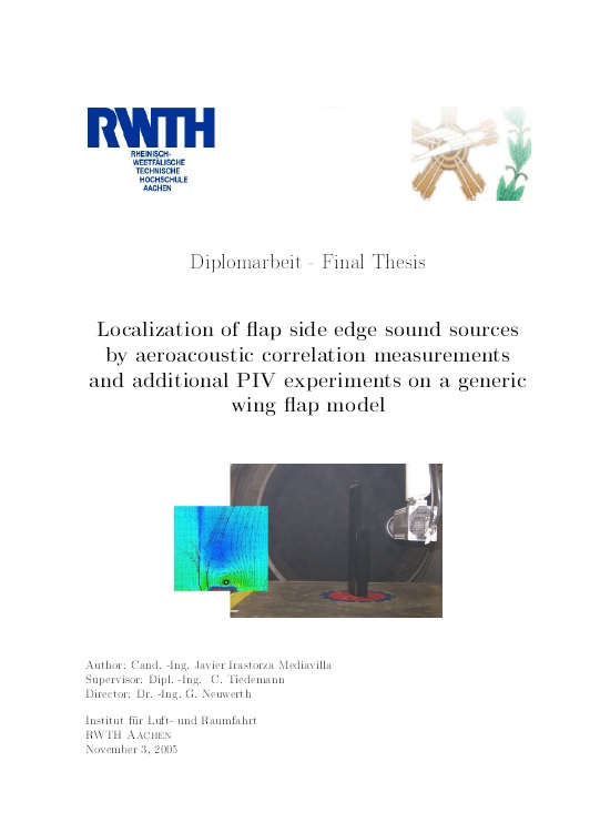
Master thesis front page.
It happens that, back in 2005, I completed my aeronautical engineering master thesis with a project carried out in a wind tunnel at the Aerospace Institute (Luft- und Raumfahrt) of the RWTH-Aachen. Those two posts brought back some good memories and I thought I could share a couple of them here in the blog. Jaime has worked in a wind tunnel in Audi, and in his posts he included some pictures from other affluent wind tunnels. You will see here the contrast with budgetary constrains lived by universities.
I think that for this post I will be brief in the comments and will focus on sharing some pictures trying to bring you about what we tried to do and how we did it. Directly, from the thesis preface:
This Diplomarbeit is the result of two different experiments. Each one is dealing with different techniques but both share a common aim: the comprehension of the noise generation in the flap-side edge. That is the reason for presenting both experiments in a very similar way in this report, so the reader might see two parallel experiments which final results are analyzed together.
Thus we wanted to measure noise and correlate it with the flow around the flap. How did we measure the noise in the vicinity? “Aha! an acoustic camera!”, and you then remember the arrays of microphones my brother displayed in his post. See here the arrangement we had:
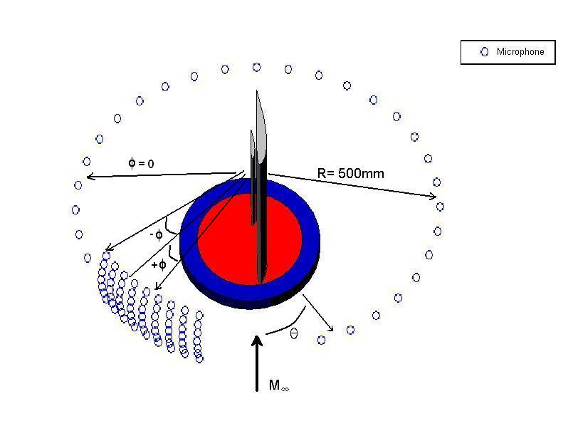
“Acoustic camera”.
Fancy, isn’t it? Except for which we indeed counted with a single micro, which we had to move to every position of the array and thus repeat long measurements endlessly. 🙂
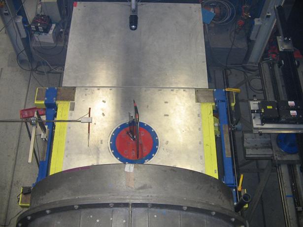
Aerial view of the experiment.
In the picture above you can see the wing profile with the single micro in the left (to the intrados of the wing).
Once we had made dozens of measurements it was just a question of letting Matlab do the dirty job and plot measurements for each position at different flap deflections…
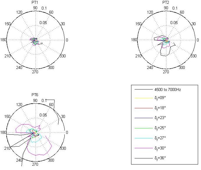
Noise measurements.
But remember that we wanted not only to measure noise but to correlate it with the flow structure at the flap edge. Let me advance you an image of what we wanted to see:
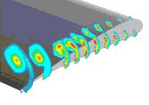
Vortex structure.
How did we make to study the flow? Another of the techniques introduced by Jaime, Particle Image Velocimetry, directly from the Wikipedia:
Particle image velocimetry (PIV) is an optical method of flow visualization […]. It is used to obtain instantaneous velocity measurements and related properties in fluids. The fluid is seeded with tracer particles which, for sufficiently small particles, are assumed to faithfully follow the flow dynamics (…). The fluid with entrained particles is illuminated so that particles are visible. The motion of the seeding particles is used to calculate speed and direction (the velocity field) of the flow being studied.
[…]
Typical PIV apparatus consists of a camera (…), a strobe or laser with an optical arrangement to limit the physical region illuminated (…), a synchronizer to act as an external trigger for control of the camera and laser, the seeding particles and the fluid under investigation.
Seeding the flow, recording it with a camera, using a laser beam… boy, doesn’t it sound fancy high-tech? Let’s go and describe it.
See a plan of the wind tunnel we used:
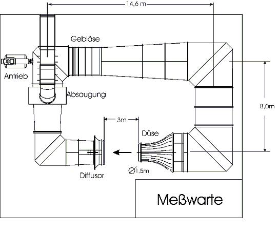
Wind tunnel plan.
See an schematic of the equipment and connections we used for the experiment, all placed at the open section of the tunnel:
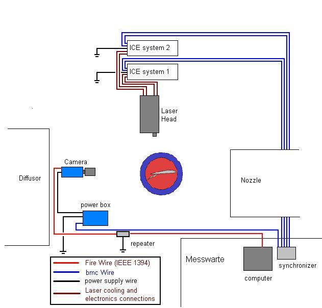
Schematic of the experiment.
See exactly where we wanted to shoot at with the laser beam:
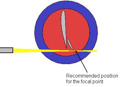
Laser bream.
See from where we recorded the images (camera at the right side of the picture, downstream from the wing):
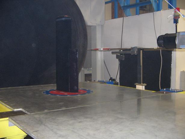
Camera.
See in this other graphic a summary of the technique. The laser emits two consecutive pulses which light the seeded particles. The camera records those 2 consecutive images and a dedicated software measures the movement of each particle thus providing the information of the flow.
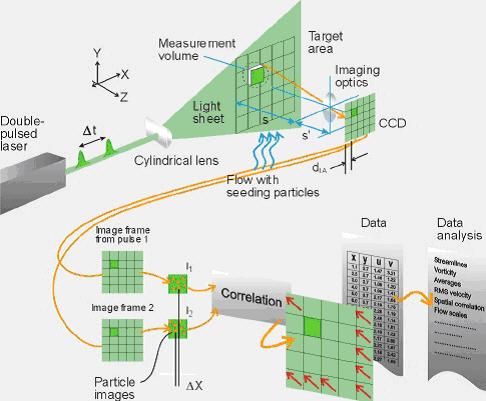
Schematic of PIV technique.
So far, so good.
However, it happens that this was the first time we were using the technique at the institute and despite of our reading of references it took us some time, trials and finally asking experienced people to pull the right strings. At the beginning we just either saw nothing or blurry images.

Blurry image.
After days of running the tunnel seeded with oil particles you can imagine the fog we were in:
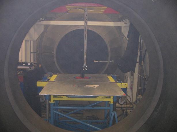
Oil fog.
… and what we needed were two consecutive shots of very well-defined particles. In the end we managed to fine tune everything and get the desired results:
Image of particles.
Once we had the images, we ran all the correlations with the acoustic measurements of our array of one microphone and had all the data to analyze, draw some conclusions, propose some new paths to continue experimenting and with which to write a nice thesis.
All that was left was to clean up the mess at the tunnel:
Cleaning the inside of the wind tunnel.
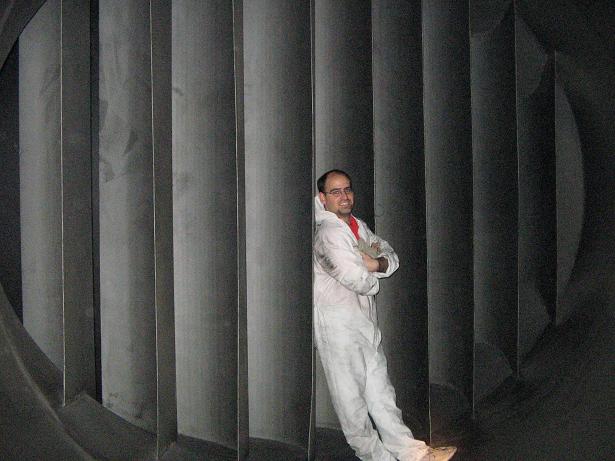
But, yeah, who’s got a picture of himself between the stator and the rotor of a wind tunnel? 🙂

Me among the vanes of the stator.

