Boeing 787, the Dreamliner, made its first commercial flight with Japanese airline All Nippon Airways between Tokyo and Hong Kong. The event has been widely covered in general and specialized press. One of such articles, in Bloomberg, was the spark of a conversation with a colleague that led to the following question: will the 787 ever bring value to Boeing? Will the net present values of all the cash flows related to the programme ever be positive?
After a conversation, I decided to try to answer to those questions, using information found in different sources across the internet.
Lately there has been much discussion in the media about what would be the Boeing’s “accounting block” size (finally it was announced to be 1,100 aircraft units). This concept refers to the number of aircraft upon which Boeing is going to spread the amortization of the work in process now in the balance sheet (around 18bn$ at 2011 Q3, according to Boeing), excluding R&D costs (which were already accounted for in previous years’ income statements).
While the concept has raised much attention, it is irrelevant to appraise the 787 as a long-term investment project, for which yearly cash flows, accordingly discounted for (to take into account the time value of money), shall be calculated. This time including R&D costs.
Together with the previous concept, last days’ news have often discussed the concept of “learning curve”. This is a concept typically used in aerospace industry and which will be central to the discussion of whether the 787 will be or not a success as an investment project.
Learning or experience curve
Let me introduce the learning curve effect by quoting directly from the Wikipedia:
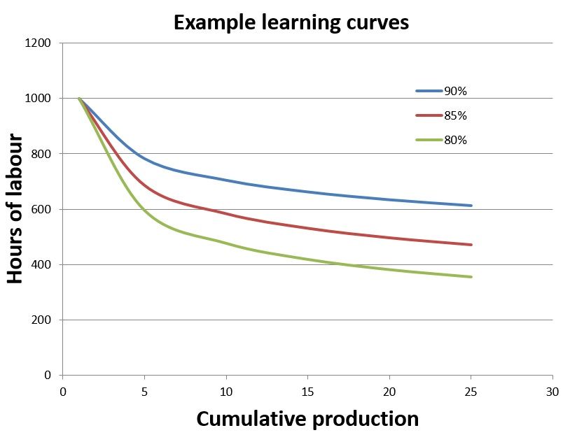
“The rule used for representing the learning curve effect states that the more times a task has been performed, the less time will be required on each subsequent iteration. This relationship was probably first quantified in 1936 at Wright-Patterson Air Force Base in the United States, where it was determined that every time total aircraft production doubled, the required labour time decreased by 10 to 15 percent.” […]
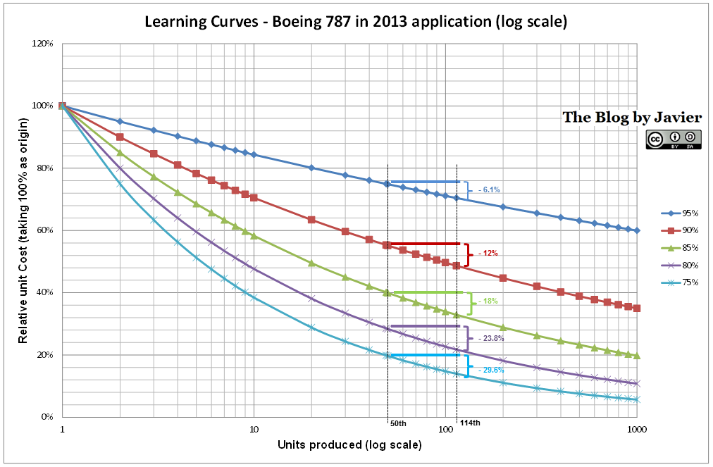
“Learning curve theory states that as the quantity of items produced doubles, costs decrease at a predictable rate.”
The press has stated that Boeing’s targeted learning curve for this programme will be 75%, despite of having less control over the supply chain in comparison with previous developments. That means that every time production units have doubled, the unit cost will have decreased in 25% (if unit 100th costs 100, unit 200th shall cost 75).
In the last new aircraft development, the 777, Boeing reportedly experienced a curve of 84% (costs decreasing 16% every time production units doubled). In this exercise I will make use of different values for the learning curve in order to see its influence (90%, 84% -as with 777-, 80% and 75% – Boeing’s target).
Discounted cash flows
Due to the time value of money, i.e. the interest that could be earned by a given amount of money, it is important to evaluate the present value of the cash flows of the 787 project along its life-cycle. As the Wikipedia states it:
“Net Present Value is a central tool in discounted cash flow (DCF) analysis, and is a standard method for using the time value of money to appraise long-term projects.”
This basic concept of finance theory is rarely covered by the press.
The then-assistant professor of Economics and Public Affairs at Princeton University, U.E. Reinhardt, in his paper “Break-even analysis for Lockheed’s TriStar: an application of financial theory” (PDF, 2001), analyzed comprehensively the project of the TriStar making use of information that became public at a moment when Lockheed officials took part in Congressional hearings over a loan-guarantee needed by the TriStar programme (1971).
Reinhardt found that the figures that appeared in the media led one to consider that the programme cash flows were not discounted either to the time at the beginning of the project or to the time of the congressional hearings, as prices and market numbers would had only produced a positive net present value if the discount rate had been in fact around 0%, that is “only if one assumes that the company was prepared to advance the enormous sums required for that project without asking for any positive return on this investment”.
Typically the discount rate used to evaluate different projects is the cost of capital of the company. For this exercise I have used different rates to see its influence in the results (0%, 5%, 10% and 12%, being the last two typical figures used in industry).
As a side note: Reinhard used as learning coefficient 77.4%, close to the optimistic 75% targeted by Boeing and lower than the disclosed 84% of the 777 case.
Data gathering
In order to build the exercise, different sets of data need to be collected. I will discuss them below, indicating the sources used and explaining the assumptions taken.
Number of aircraft produced
According to news reports, this year Boeing will deliver between 15 – 20 787 and 747-8, being about two-thirds of the latter. From that information I took that about 6 787s will be delivered in 2011. From then on, the ramp I used tries to replicate what the media is reporting.
Boeing intends to reach a rate of 10 aircraft per month by end 2013, thus from 2014 I assumed Boeing will produce 120 787s every year (as Boeing factors down time into calculation of the monthly rate).
According to Seattle Times, this week Boeing is increasing its rate from 2 aircraft per month to 2.5. Since between 2012 and 2013 this rate has to increase from 2.5 to 10, I assumed an average of 3 aircraft/month for 2012 and 6 for 2013.
Number of aircraft sold
Boeing publishes in its website the number of aircraft ordered each year. For this exercise, I took into account the net orders in the year of order.
In the last conference call, Boeing stated that it sees an addressable market for the 787 in the next 20 years of 5,000 aircraft (this number of aircraft reflects deliveries). As of today, Boeing has close to 800 orders. This backlog covers the production until somewhere in 2019, in order to keep the production line with a steady production rate, I assumed Boeing will sell the necessary aircraft to allow a steady state production of 120 aircraft per year until the end of the exercise in 2034. That would mean Boeing would have delivered 2,634 aircraft, a bit over half of the 5,000 aircraft that represents the addressable market.
Since Boeing has already sold close to 800 of those 2,634 aircraft, I assumed the rest will be sold evenly every year, or at a rate of 82 aircraft per year from 2012.
List price of the 787
Boeing publishes in its website the list prices of all its models. The list price of the 787 today ranges from 193.5 to 227.8 million USD, or about 211 M$ on average.
At the end of 2010, Boeing raised its list prices 5.2% on average. The previous raise had taken place in 2008, 2.6% in relation to 2007 prices, when they had been raised another 5.6% after two years.
From those numbers, I made the assumption forward and backward that on average Boeing raises its list prices about 2.6% per year.
Price discounts
I have already published two different posts about average Boeing price discounts for 2009 and 2010. A recent article from Flight Global confirmed the order of magnitude for the case of the A380. The discount rate I used for the exercise is 38%.
Another confirmation of the order of the discounts specifically for the 787 comes from the following analysis by Jon Ostrower, from Flight Global, who reports prices of 787 to be around 76M$ in 2004-2006, excluding engines, which were about 20-30M$ (a total of 96-106M$).
Taking the list prices above for those years and using the 38% discount for that period of 2004-2006 the real prices given by my model are in the order of 101-104M$, in the same order that Jon’s information.
Down payment
Here I used for the exercise the same assumption I had used to calculate Boeing discounts in previous posts: a single 3% down payment taken from the AIAA paper “A Hierarchical Aircraft Life Cycle Cost Analysis Model” by William J. Marx et al.).
Regarding down payments, I once received another input in my blog from the analyst Scott Hamilton (Leeham), where he mentioned several progress payments of 3-5% of the price of the aircraft so that at the time of delivery 30% of the aircraft had already been paid for. Simulating these payments complicates the model, but, since early cash inflows may have an impact in the break even analysis, I have checked the variation with different sizes of down payment (3%, 20%).
Costs
These are the main inputs needed for the whole analysis. Most of the non-recurring cost (NRC) have already been incurred, thus, there is little room for manoeuvre in there. However, regarding the recurring costs (RC), those are where Boeing has the chance to make the programme profitable.
NRC: Research & Development (R&D) and capital expenditures (CAPEX)
Seattle Times provided a detailed description of the incurred costs that Boeing had through end September 2011. The account was split in different categories of non-recurring costs (R&D, CAPEX, buying out partners) totalling over 16bn$.
RC: Inventory, advances to suppliers
In the same article there was another explanation about the recurring costs (inventory –work in process, supplier advances and others) incurred so far: up to 16.3bn$ by September. This last figure has risen to 18bn$ according to the last conference call given by Boeing.
In order to build the cash flow profile, it is necessary to know the cash flow profile of the costs described above. Since we have only information regarding some of those (buyout of partners, CAPEX for Charleston FAL) I needed to make an assumption for the rest.
In this case, I used the same cash profile used by B. Esty and P. Ghemawat (both then at Harvard Business School) in their paper “Airbus vs. Boeing in Super Jumbos: A case of failed Preemption” [PDF], where they performed a valuation analysis for then known as A3XX (now A380).
You may see in the following graphic the cash profile used up to now:

Boeing 787 costs through 2011 profile.
Regarding the recurring costs, the main finding to be done is the recurring cost of the aircraft at a certain point. Once we have a reference, we can play with the learning curve to see how the costs will be in the future or were in the past.
Different sources quote figures as 250-300M$ or even 400M$, but they do not explain whether that is the cost of a unit right now (e.g. serial number 44) or whether it is the average cost up to now (they do not indicate how many aircraft are included in that average either if that was the case).
The approach I followed was different.
Boeing has disclosed it has 18bn$ as WIP related to the 787, and from local press we know what is the state of production right now, thus, we can try to estimate what is the average cost of the aircraft already produced.
The aircraft delivered to ANA needs to be discarded as its portion of WIP has already been included in the income statement of Q3. We know that at Seattle FAL there are now serial numbers 46 (to be completed according to press) to 50 (just arrived, according to Jon Ostrower). Thus, within WIP there must be about 44 aircraft almost completed and another 5 about 98% completed (FAL value added is around 4% of RC).
As we do not know how many other aircraft are in process and at which stage each one, we need to make further assumptions. From the same article of Seattle Times we learnt the following:
“The first 40 out of the Everett factory required massive and repeated rework, and the next 10 to 20 also need modifications because of design changes after flight testing.”
That means that at least about another 20 aircraft are being manufactured when other aircraft are at FAL. We can assume an average stage of completion of 50% of costs incurred in each one. With these assumptions, we gather that the 18bn$ correspond to about 58 aircraft in different stages of work in process (WIP).
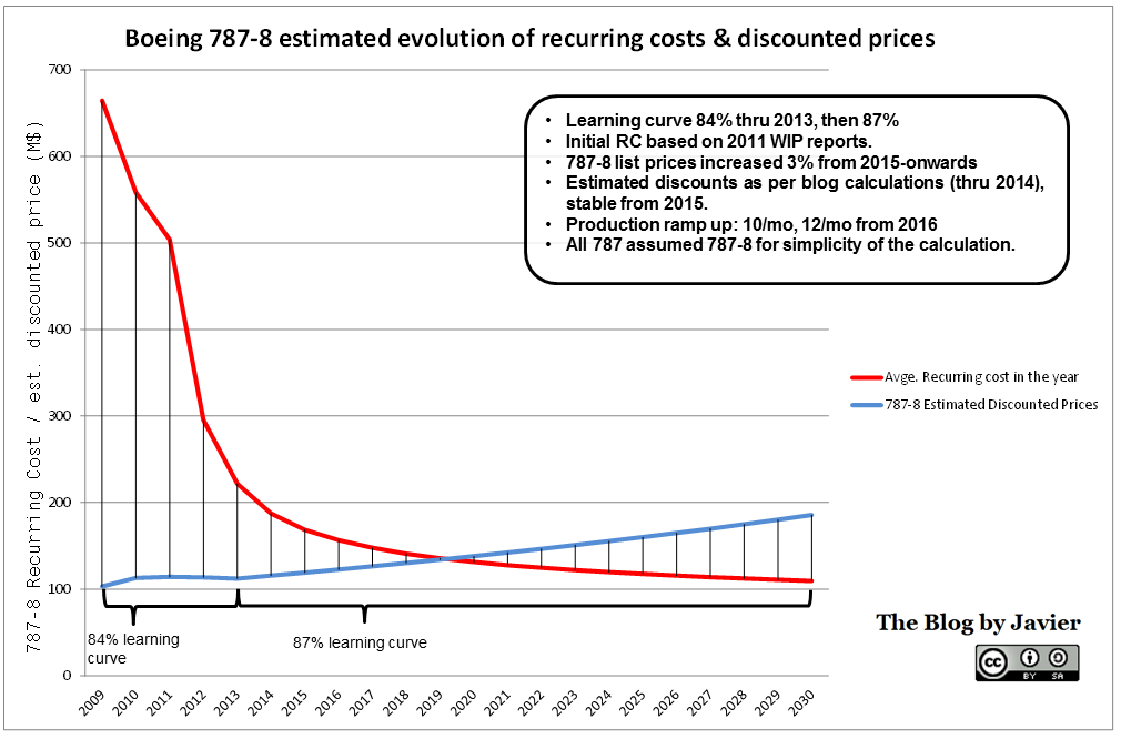
This gives us an average cost of about 310M$ apiece, close to the figures mentioned by some sources. The difference is that now we have a reference of cost and aircraft unit or units for that cost (1 delivered + 44 finished + 5 at FAL + 10-20 WIP ~ 60-70 aircraft).
With this average cost and using the learning curve formulas, we can deduct the unit cost of the first unit produced, which will be different for each learning curve we select, and from which all the costs of future units will be calculated.
Side note: Both 80% and 75% curves yield lower unit costs than the aircraft price (with the 38% discount) by the year 2015, in line with what was disclosed by Boeing CFO James Bell during the conference call:
“Bell projected that the cost to build each Dreamliner will drop below the price paid by the buyer around 2015, providing positive cash flow for the first time.”
Analysis
With all the data gathered above, and the required assumptions made, we can build a comprehensive valuation analysis.
Boeing 787 will not break even before 2034
The first graphic that is shown is what I believe will be the real scenario for the 787: it will not break even in the first 30 years of the programme, discounting cash flows. It won’t break even before 2034. In this case, I used the learning curve of 84%, that which was reported as the real one for the 777, and which is more conservative than the targeted one, 75%. As discount rate for the cash flows I used 10%, which could be even considered a bit low.

787 cash profile for a learning curve of 84 and discount rate of 10%.
When will then the 787 break even?
I continued the series for this set of reference parameters (84% curve and 10% discount rate) and break even would indeed happen, but not before 3650 units of the 787 have been delivered at the year ~2046. By then production rate would have had to slow down to about 6-7 aircraft per month as the backlog would have been already consumed, thus a new cost structure per unit produced could even make the mentioned date to be deferred even later.
Influence of the discount rate
The discount factor could be assimilated with the cost of capital. The reference I used was 10%, but let see how the previous graphic would look like in the case the factor was lower 5% and a bit higher 12%.

787 cash profile for a learning curve of 84% and discount rate as parameter.
We can see that if the cost of capital was as low as 5%, the 787 would reach break even by around 2028, but in the case of 12% it would never break even within 30 years as well.
Influence of the learning curve
The learning curve I used was the one I believe is more realistic as previous Boeing’s experience has shown, 84%. But let’s see how it influences the valuation, now fixing the discount rate at 10% and using the learning curve as a parameter:

787 cash profile for a discount rate of 10% and learning curve as parameter.
We can see that if the curve is the 90% the outlook is much darker, however, for 80% the programme would break even within the first 30 years, at around 2029. If the curve is the one Boeing targets, 75%, the programme may break even at around 2023, in line with Boeing statement:
“The positive cash flow will gradually pay back the earlier production costs to finally break even on manufacturing the planes roughly 10 years from now, Boeing said.”
Influence of the discount in prices
I have used a 38% discount over prices. I feel quite confident that Boeing discounts are around that figure, nevertheless, let’s see what would happen to the reference case (84% curve) if discounts were just ~20%, about half of those used, which would make cash inflows much higher at the moment when deliveries start.

787 cash profile for a learning curve of 84%, discount rate as parameter and discount over price of 20%.
We can see that in that case, the break even would be within the first 30 years, at about 2024 already for a DCF discount rate of 10%. Nevertheless, I doubt that pricing power of Boeing will allow it to stop giving ~38% discounts.
Influence of the down payments
In the simplified case that the down payment at the time of ordering the aircraft wasn’t in the order of 3% but 20%, this would bring forward cash inflows especially related to the first 800 aircraft ordered and thus improve the business case. However, once the programme is in steady state it wouldn’t change much.
You may see that maximum cumulative negative cash flow for the 5% curve only reaches about ~19bn$ vs. ~32bn$ in the reference case. Also for the 5% curve the break even is brought forward 2 years (from 2028 to 2026).

787 cash profile for a learning curve of 84%, discount rate as parameter and down payment of 20%.
“Boeing’s view” on the matter?
As we have discussed above, Boeing is targeting a learning curve of 75%, ambitious if compared to that of the 777, but not far from that used by Reinhard in his paper.

"Boeing's view": 787 cash profile for a learning curve of 75%, discount rate as parameter.
In this case, you may see that with a discount rate of 10% break even is reached in 2023. Again, as mentioned above, this is in line with Boeing’s comments in the conference call. Even for a discount rate of 12% break even would come within the next decade at around 2026.
This stresses the importance of the learning curve effect and cutting costs during the series production phase. Being in the state that the programme is now, with about -22bn$ cumulative cash flows through 2011, the only way to save it is through experience gained at the production sites.
The question then is: Will Boeing be able to achieve that 75% curve?
Side note: Let me now come back to the price discounts. I find that the results shown in the last graphic, with the curve Boeing intends to achieve (75%) and a discount rate for cash flows of 10%, as another confirmation of the discount used for prices of aircraft.
The model I built takes the 38% figure discounted from list prices, and I find it remarkable that with that figure the model predicts lower unit costs than aircraft discounted prices by 2015 (as mentioned by the CFO, James Bell) and predicts a programme break even at around 2023, about 10 years from now, as mentioned in the conference call. I take the last conference call as an implicit confirmation from Boeing of the discounts it applies to its 787s.
What has been the effect of this 3-year delay?
This is not easy to estimate, but I’ll give it a try.
Most of the assumptions remain constant. I believe that the delay has primarily deferred cash inflows from deliveries, extended R&D related to engineers working in the development for 3 years more sorting out problems and increased WIP of aircraft waiting in the production line. I will also remove cash spent in buying out partners, though this might be arguable as possibly the price of the buyout is cash neutral taking into account partners’ margins disappearing.
Below you may see the two graphics, one for the reference case (84% curve) without delay and the other for Boeing’s target (75%):

Effect of 3-year delay to 787 cash flows for learning curve of 84%.

Effect of 3-year delay to 787 cash flows for learning curve of 75%.
You may see that even in the conservative scenario (84%) break even is reached in 2014 or 2015 depending on the discount rate. With the more aggressive learning curve, 75%, the prospect is even rosier: from 2013 for both discount rates the programme would have reached break even less than 10 years since its launch in 2004 and 10 years before what now seems to be Boeing’s target break even year, 2023.
This result clearly points out how much a delayed programme may hurt the business case of an aircraft development: from being a sound project to converting it into a nightmare that may never break even, jeopardizing future developments in terms of lack of financial and human resources available.
What is the “accounting block” size used for then?
As its name points out, this is a mere accounting issue. It permits Boeing to spread already incurred costs that have been capitalized (in the balance sheet, not in previous years’ income statements) among aircraft to be delivered in the future. Since Boeing has a backlog of almost 800 aircraft and believes it will sell over 2,500 aircraft, it has prudently opted to spread costs over 1,100 aircraft, allowing itself to start reporting profits on each aircraft delivered almost from day one (from about 2015 in fact), having a shinier income statement and the bonuses that come with it.
—
Finally, as Richard Aboulafia would put it:
“Yours, ‘Til The 787 Breaks Even”