Monthly Archives: November 2026

Bartolomeu Dias and the passage of the Cape of Good Hope

“The discovery of America, and that of the passage to the East Indies by the Cape of Good Hope, are the two greatest and most important events recorded in the history of mankind.”

“What benefits or what misfortunes to mankind may hereafter result from those great events, no human wisdom can foresee.”

Adam Smith, The Wealth of Nations (1776), Book IV, Chapter VII

I come back very often to this quote, typically around Columbus day (October 12th) or when discussing the discovery of America. In this post I wanted to focus on the passage to the East Indies by the Cape of Good Hope, who opened it, how it happened, and what the route looks like today, with some data on trade and ships.

Portuguese exploration along the African coast accelerated under Prince Henry the Navigator in the early 15th century. The goals were practical and ambitious: find a sea route to the spice markets of India, reduce dependence on Muslim-controlled land routes, and expand trade and Christian influence.

Bartolomeu Dias, the man who opened the route

Very little is known about his early years. Bartolomeu Dias was born around 1450 in Portugal, probably into a family with a maritime tradition. He served at the court of King John II (João II) as a cavalier of the royal household and superintendent of the royal warehouses, and in 1481 he is believed to have taken part in Diogo de Azambuja’s expedition to the Gold Coast (modern Ghana) to establish the fortress and trading post of São Jorge da Mina (Elmina). In October 1486 he received an annuity from the king for “services to come”.

In 1487 the king commissioned him to continue the exploration of the African coast beyond the points reached by Diogo Cão, and to seek a sea route to Asia. He left Lisbon in July or August 1487 with three ships: two caravels of about 50 tons each (São Cristóvão, captained by himself, and São Pantaleão) plus a supply ship commanded by his brother Diogo. Some key points of the voyage:

  • He sailed down the West African coast past Cão’s markers, reaching Walvis Bay (Namibia) around 8 December 1487.
  • Driven southwest by storms (or deliberately sailing) into the open South Atlantic, he traced a wide arc well west of the African coast.
  • First landfall east of the cape: around 3-4 February 1488, at what is today Mossel Bay (South Africa). Without knowing it, he had already rounded the southern tip of Africa.
  • He continued east to Kwaaihoek, near the mouth of the Bushman’s River, where on 12 March 1488 the crew planted a padrão (stone pillar) dedicated to St. Gregory.
  • There the exhausted crew forced the return. On the way back they finally sighted the cape itself (May 1488). Dias reportedly named it Cabo das Tormentas (“Cape of Storms”); King John II later renamed it Cabo da Boa Esperança, “Cape of Good Hope”, because it promised a route to the East.
  • He arrived back in Lisbon in December 1488, some 16 months later, having charted hundreds of miles of previously unknown coast.
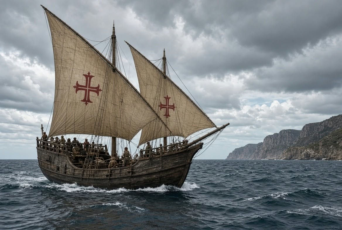
A Portuguese caravel with lateen sails bearing the Cross of the Order of Christ, at sea off a rocky coast
A caravel of the kind Dias sailed in 1487-88, lateen sails bearing the Cross of the Order of Christ (AI image by Grok)

After his return he received limited recognition, but he helped design and outfit the ships (São Gabriel and São Rafael) for Vasco da Gama‘s 1497-1499 expedition to India. In 1500 he commanded a ship in Pedro Álvares Cabral’s fleet bound for India and died on 29 May 1500, when a storm sank four ships near the very cape he had first rounded twelve years earlier. Contemporary records of his voyage are scarce (many were lost in the 1755 Lisbon earthquake); much of what we know comes from later chroniclers such as João de Barros.
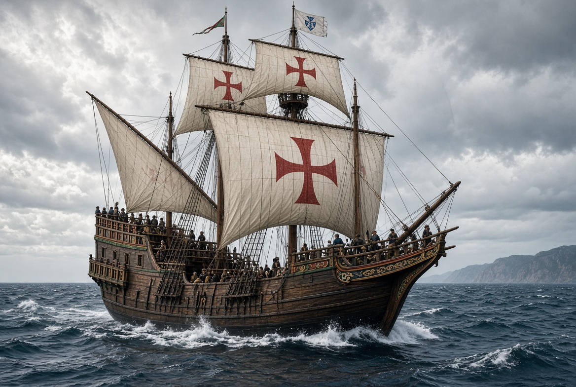
A Portuguese nau (carrack) under square sails bearing the Cross of the Order of Christ
A nau like da Gama’s São Gabriel (1497); Dias superintended the building of da Gama’s ships (AI image by Grok)
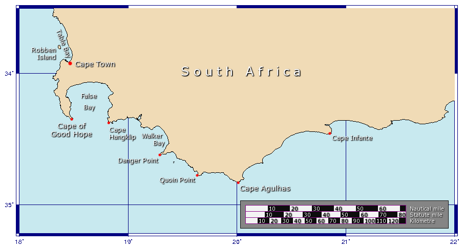
Map of the Cape of Good Hope region, South Africa
The Cape of Good Hope and the neighbouring capes (Cape Agulhas is the true southern tip of Africa). Map: Johantheghost, Wikimedia Commons, CC BY-SA 3.0.
Cape of Good Hope, Cape Town, South Africa

A school project (and a family trip)

This is a subject we know well at home, as earlier this year when my daughter Andrea (then 12 years old and studying in grade 7) had to do a school project for History class, she chose to do it about Bartolomeu Dias, as they had been studying trade routes, the Silk road, etc.

School project poster about Bartolomeu Dias
My daughter’s school project on Bartolomeu Dias.

Her poster covers who sent him south (King John II), who accompanied him on the journey, the effect of the expedition on the world, and the four places where, according to her research, he left his crosses: Cape Negro, Cabo Voltas (both on the way south), the Cape of Good Hope, and Kwaaihoek / Algoa Bay on the way back. And she proudly notes: “I have actually visited one of Bartolomeu Dias’s Crosses (Padrão’s) in Namibia“.

Indeed. On a family road trip around Namibia in 2024, we stopped at Dias Point, near Lüderitz, where a replica of that padrão still stands:


Family selfie at the Dias cross in Dias Point, Namibia
At the Dias cross, Dias Point (Namibia).
The kids at the coast by Dias Point
The kids at Dias Point. The wind helps understand why Dias first named it Cape of Storms.

The information board at the site tells the story well: on 25 July 1488, on his way back to Lisbon, Dias was forced by strong headwinds to anchor in a bay he named Angra Pequena (26°38′ S, 15° E, today’s Lüderitz), where he raised a padrão dedicated to São Tiago (St. James). The original cross eroded away; in 1953 the historian Eric Axelson found fragments of it at Dias Point, and in 1988, for the 500th anniversary of the voyage, a replica sculpted from Namib dolerite was unveiled there.
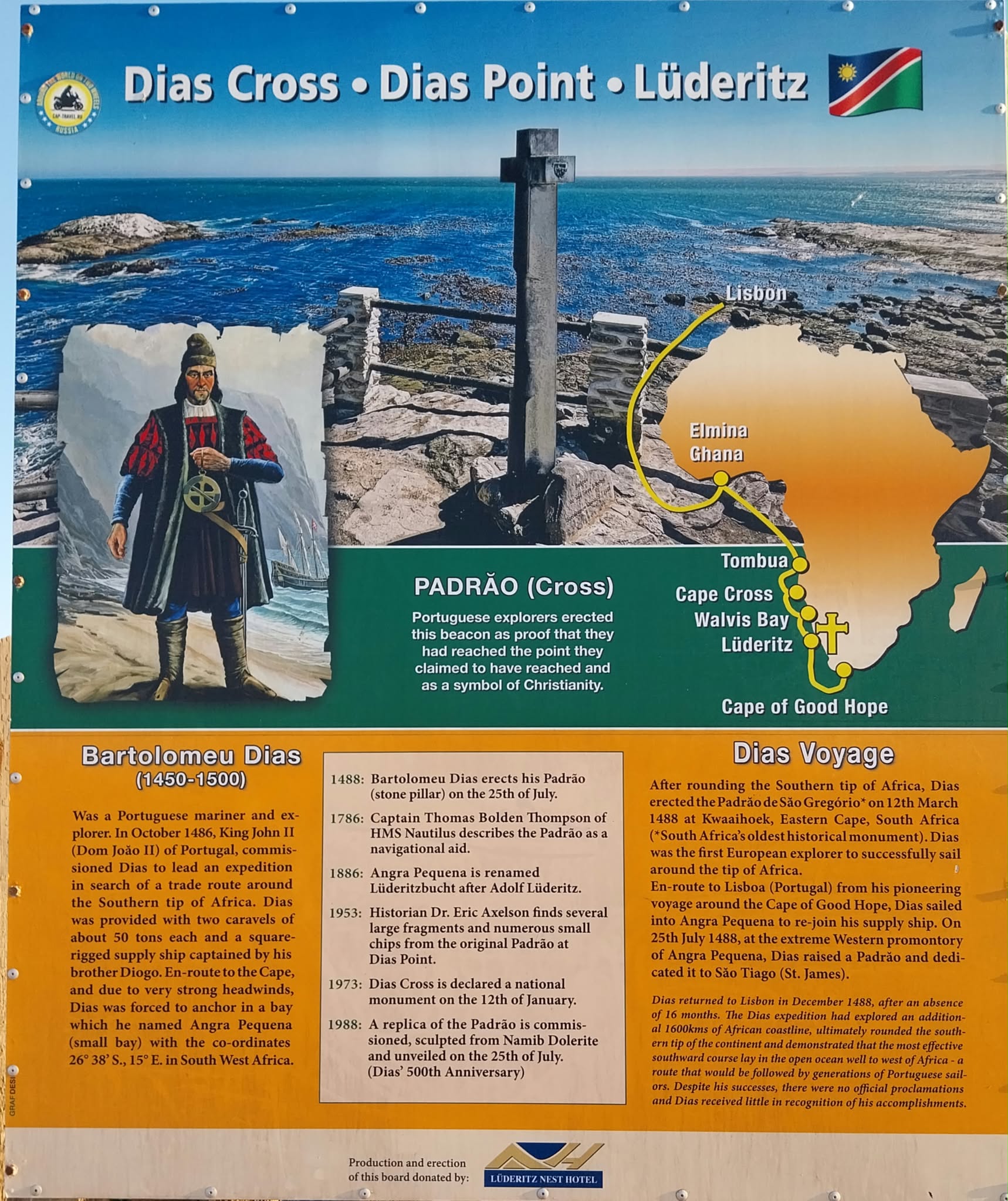

Information board at Dias Cross, Dias Point, Lüderitz
Information board at Dias Cross, Dias Point, Lüderitz (Namibia).
Replica of the padrão raised by Bartolomeu Dias at Dias Point
The padrão replica (1988) at Dias Point.

Was Smith right? The Cape route in today’s trade

Let’s look at some data. Over 80% of world trade by volume moves by sea, according to UNCTAD. World merchandise exports were worth about $24.4 trillion in 2024 (WTO), against a world GDP of roughly $112 trillion in 2024 and some $118 trillion estimated for 2025 (IMF / World Bank). Air freight is marginal in volume, though significant in value.

And how much of that trade goes around the Cape of Good Hope?

  • Between 2015 and 2023, some 12.9%-14.8% of global dry bulk cargo (iron ore, coal, grains) rounded the Cape each year, according to URSA Shipbrokers data. The Suez Canal, the northern alternative, carries about 12% of global trade and some 30% of container traffic: over $1 trillion of goods a year on around 50 ships a day.
  • Since the Houthi attacks on Red Sea shipping started in late 2023, traffic diverted massively to the Cape: dry bulk cargo via the Cape rose to 19.1% of the global total in 2024 and 20.4% in the first half of 2026 (583.5 million tonnes out of about 2.86 billion).
  • Oil flows around the Cape rose nearly 50% with the diversions: from an average of 5.9 million barrels per day in 2023 to 8.7 million barrels per day in January-May 2024 (EIA) (that is 6 to 8% of world oil production, see this previous post I wrote on 2025 world oil picture).
  • Daily transits around the Cape averaged 42-56 ships per day in 2023 and 80-98 per day through 2025 and 2026 (86 in September 2026, the latest month available), on IMF PortWatch data: close to double the pre-crisis level.
  • For a typical Asia-Europe voyage, going around the Cape adds some 3,000-3,500 nautical miles and 7-10 days (World Bank); for a tanker from the Arabian Sea to Europe, the EIA puts the extra time at about 15 days.
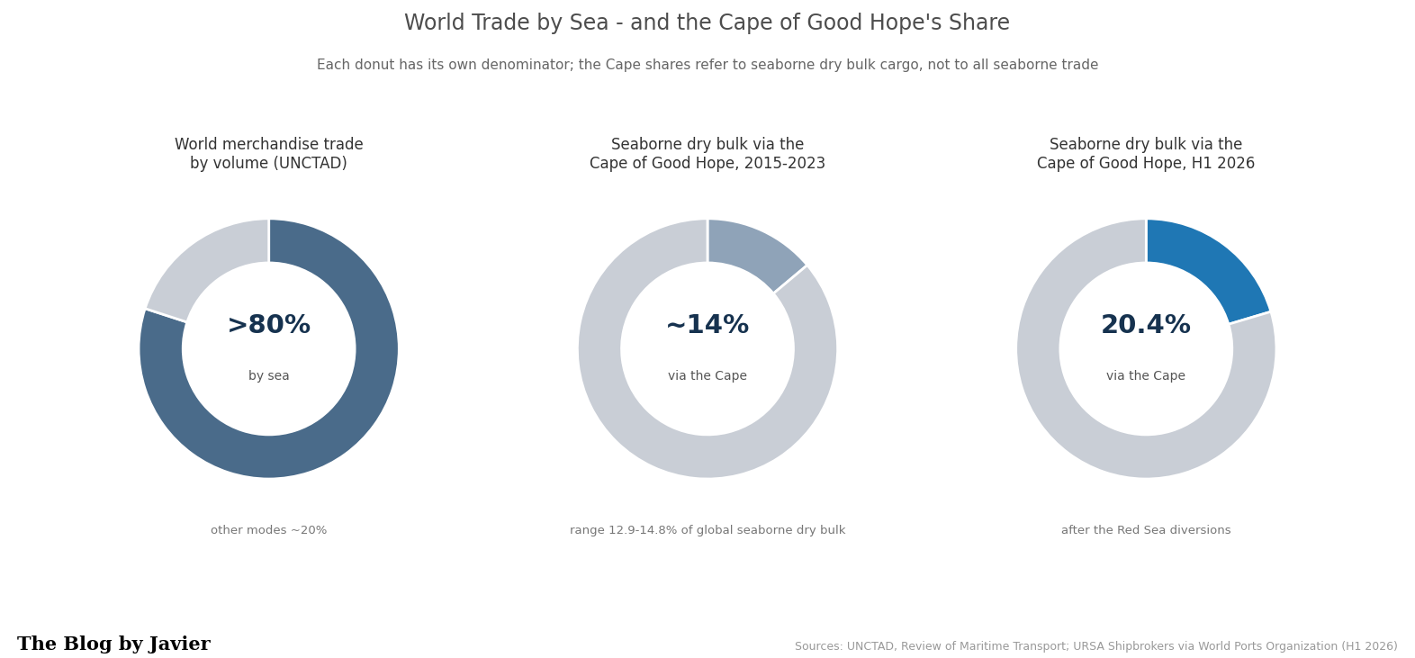
Donut charts: over 80% of world merchandise trade by volume moves by sea; seaborne dry bulk via the Cape of Good Hope rose from about 14% in 2015-2023 to 20.4% in H1 2026
Over 80% of world merchandise trade by volume moves by sea (UNCTAD); the Cape shares refer to seaborne dry bulk cargo only (URSA Shipbrokers via World Ports Organization).

In dollar terms: it is hard to give a precise bake for the Cape specifically. Pre-crisis Suez traffic was often estimated at over $1 trillion in goods value per year. The diverted portion of that, plus structural Cape bulk, represents a large absolute value, though bulk commodities have lower value density than containers. Extra costs from diversions (fuel, time, higher freight rates, insurance) have been substantial—tens of billions in aggregate higher logistics costs in the peak disruption years—but the underlying cargo value itself is in the hundreds of billions to low trillions annually depending on the exact mix and period. Even $1 trillion is only around 1% of a $112 trillion world economy. The comparison is just an order of magnitude: GDP measures value added produced in a year, while trade figures count gross cross-border sales, partly double-counted along supply chains. But the key point stands: the route Dias opened 538 years ago remains the flexible open-sea alternative (no locks, no canal tolls) that keeps world trade moving when the northern chokepoints fail.

Capesize: the ships named after the cape

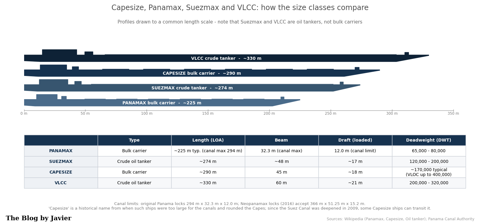
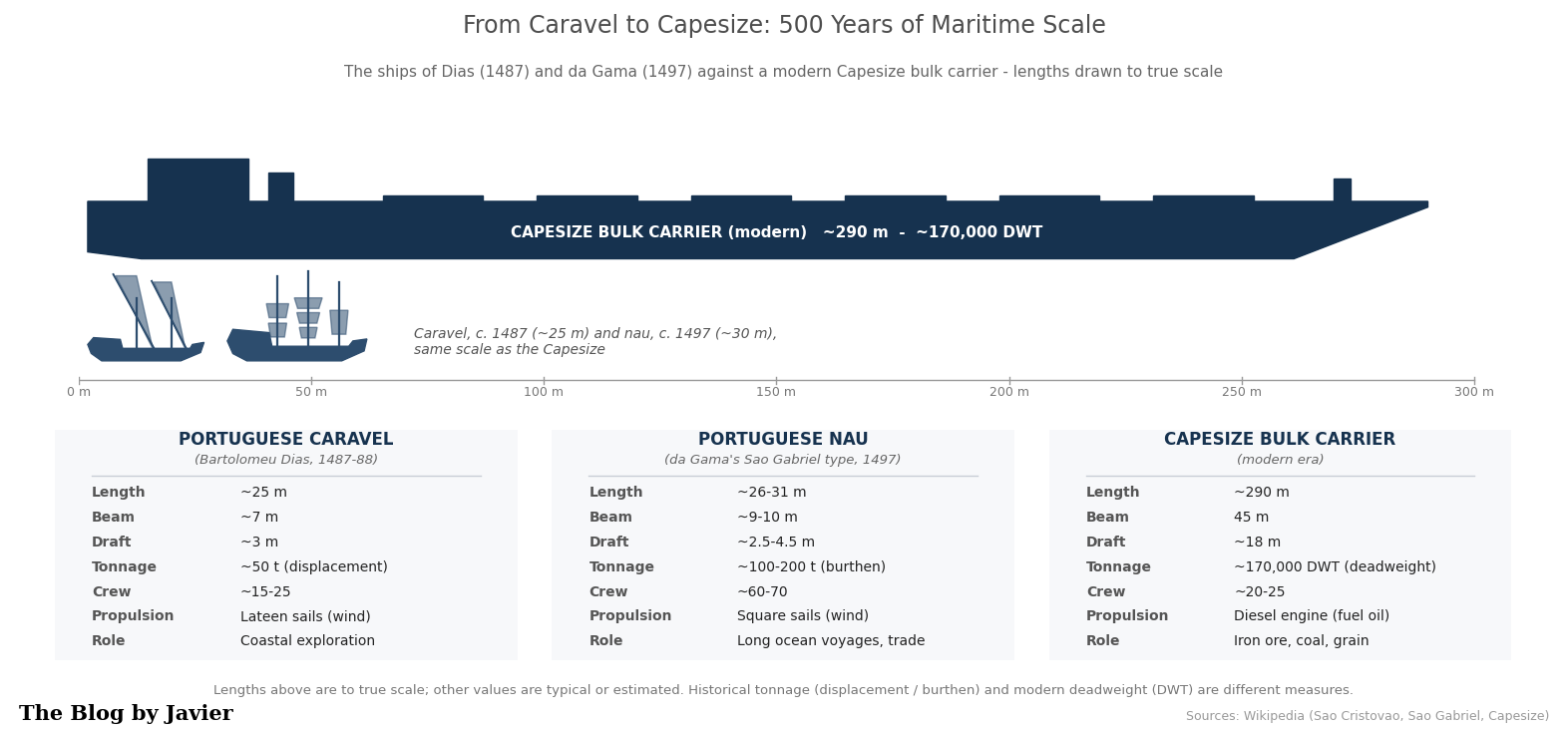
The Cape even gave its name to a whole class of ships. Capesize vessels are large dry bulk carriers of about 100,000-200,000+ deadweight tonnes (DWT), typically around 150,000-170,000: some 290 m long, 45 m of beam and 18 m of draft. They carry mostly coal, iron ore and other raw materials, and their size and deep draft mean that only the largest deep-water terminals can handle them. They were named for being too big for the canals: to move between oceans they had to go around the Cape of Good Hope (or Cape Horn). Since the Suez Canal was deepened in 2009, many Capesize ships can transit it, but the name stuck, and the Cape route remains their natural highway.
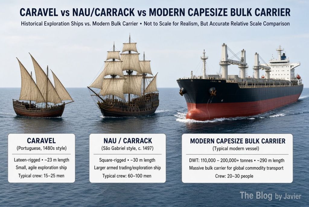
AI Grok comparison of a caravel as the one used by Bartolomeu Dias, a Nao as the one used by Vasco da Gama and a Capesize ship
Caravel (~25 m) and nau (~30 m) drawn at true scale against a modern Capesize bulk carrier (~290 m)
From Dias’s caravel (~25 m) and da Gama’s nau (~30 m) to a modern Capesize (~290 m): lengths drawn to true scale.

How do Capesize ships compare to other common ship classes?

ClassTypical DWTMain typeKey constraint / route note
Panamax~60-80k (up to ~120k Neopanamax)Bulk / tankerSized to the Panama Canal locks
Suezmax~120-200k (typical ~160k)TankerLargest tanker class transiting Suez fully laden
Capesize~100-200k+ (typical ~150-170k)Dry bulkNamed for the Cape route; after the 2009 Suez deepening many can use the canal
Newcastlemax~185-210kDry bulkUpper end of Capesize; sized to the Port of Newcastle (50 m beam)
VLCC~200-320kCrude tankerVery large crude carrier
Valemax / VLOC~380-400kOre carrierLargest bulk carriers built; deep-water ore terminals only
Panamax, Suezmax, Capesize and VLCC profiles drawn to a common length scale, with a table of typical dimensions and deadweight
The main size classes at a common length scale; Suezmax and VLCC are oil tankers, not bulk carriers.
Key dimensions of main classes of ships.

Which are the largest shipping companies in the world?
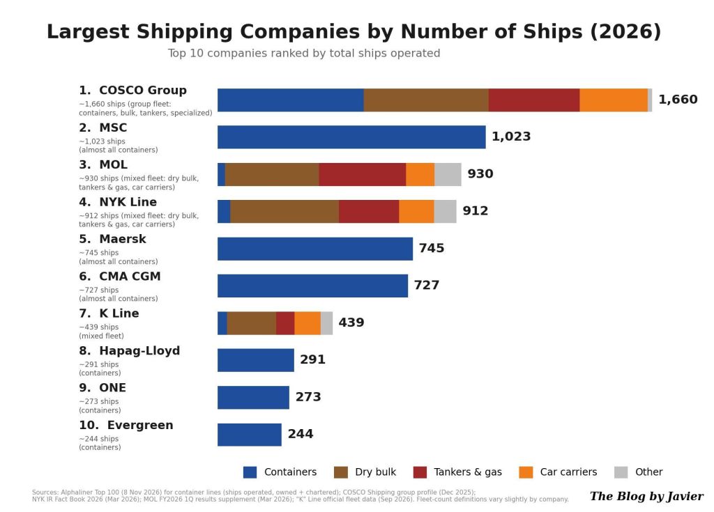
Infographic created by Instinct

The ports that receive them

Capesize ships can only call at the largest deep-water terminals, and they usually carry iron ore, coal and other raw materials, so this trade is highly concentrated between a relatively small number of specialized ports. A few characteristic examples:

On the loading (export) side:

  • Port Hedland (iron ore, Australia): one of the largest iron ore loading ports in the world and the largest in Australia. Newcastle (coal, Australia): the world’s largest coal export port, which gives its name to the Newcastlemax subclass.

On the discharge (import) side:

  • The deep-water iron ore terminals of China, which takes over 70% of world seaborne iron ore imports.

Back to Adam Smith

In the quote I shortened Smith’s sentence to “No human wisdom can foresee the benefits”. In the book, the full sentence reads: “What benefits or what misfortunes to mankind may hereafter result from those great events, no human wisdom can foresee”, and Smith himself stressed that for the natives of the East and West Indies the commercial benefits had been “sunk and lost in the dreadful misfortunes” those events occasioned.

Ten years after Dias, Vasco da Gama reached India using his route and his know-how. More than five centuries later, around ninety ships a day round the Cape of Good Hope keeping the world economy supplied, and whole classes of ships and port networks exist because of that passage. Dias received little recognition in his lifetime and died at sea next to the cape he had opened. Not a bad legacy for a “Cape of Storms”.


Sources and further reading

Note: figures come from the sources listed above; where estimates differ between sources or years, I give the ranges.
Leave a comment

Filed under Economy, Travelling, Uncategorized

Airbus vs Boeing; market capitalization since the A320neo launch (2010-2026)

In March 2024 I wrote a quick post comparing the market capitalizations of Airbus and Boeing, when I realized that Airbus had overtaken Boeing. That post compared two snapshots in time: end of 2012 and March 2024. This post shows the figures for the complete period of time since the launch of the A320neo, on December 1st, 2010, until the end of October 2026: weekly stock prices, shares outstanding, the dollar-euro exchange rate, and the resulting market capitalizations in US dollars.

Methodology in short: weekly averages of daily closing prices (Friday-ending weeks), Airbus in euros at Euronext Paris (AIR.PA), Boeing in dollars at NYSE (BA), and the FRED DEXUSEU dollar-per-euro rate. Market capitalization each week is price times shares outstanding (times the exchange rate for Airbus). Shares outstanding are forward-filled from reported figures, so early years are approximate. Sources are listed at the end.

Stock prices

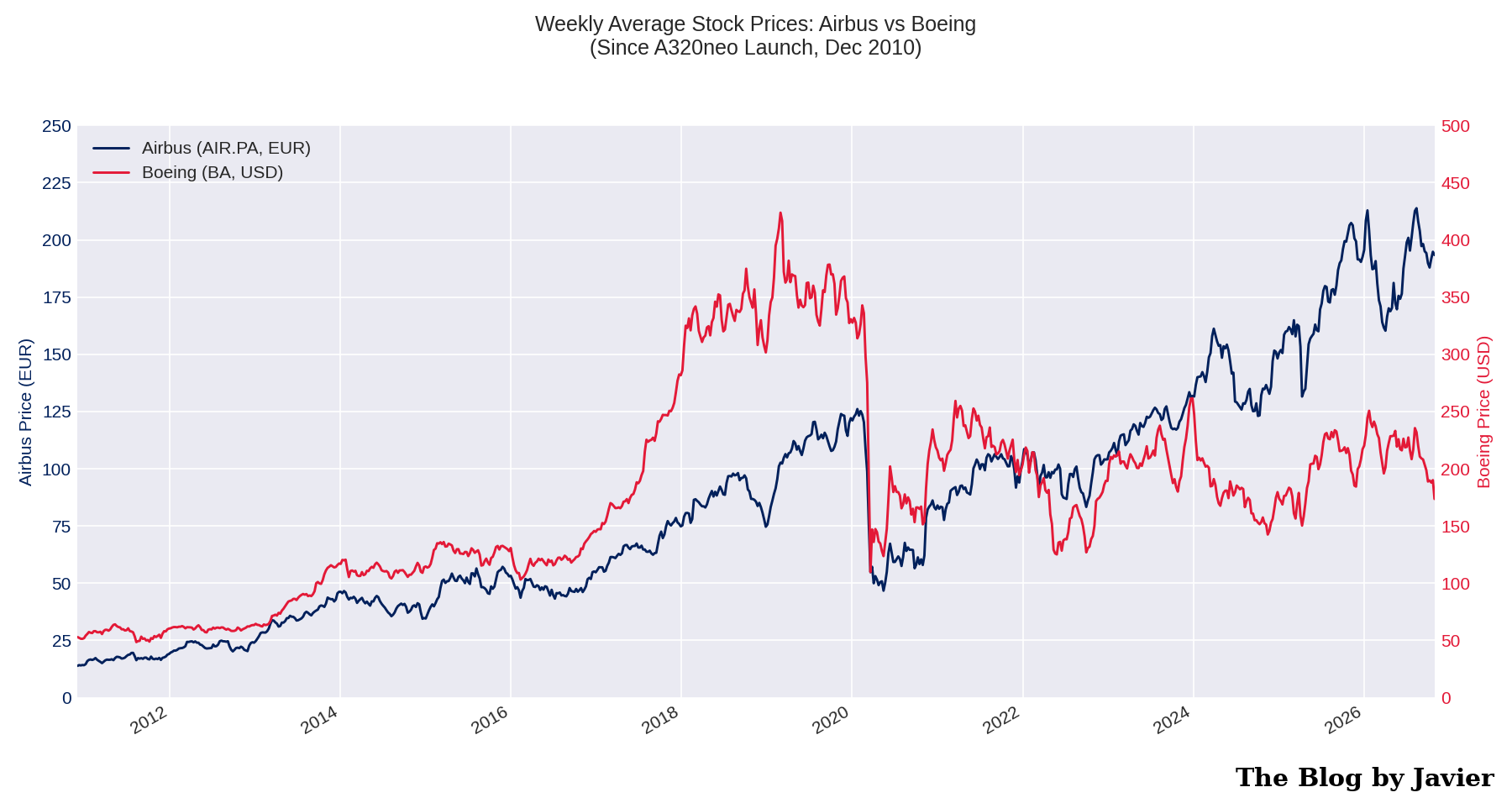
Weekly average stock prices of Airbus (EUR, left axis) and Boeing (USD, right axis) since December 2010

Airbus went from ~13.9€ in early December 2010 to ~193€ at the end of October 2026: multiplied by 14 (~18% compounded annual growth rate).

Boeing went from ~$53 to ~$174: multiplied by 3.3 (~7.8% CAGR).

Boeing peaked above $400 in early 2019, just before the 737 MAX grounding, and has never recovered those levels. Airbus suffered a milder COVID dip and resumed climbing to record levels above 200€ in 2026.

Shares outstanding

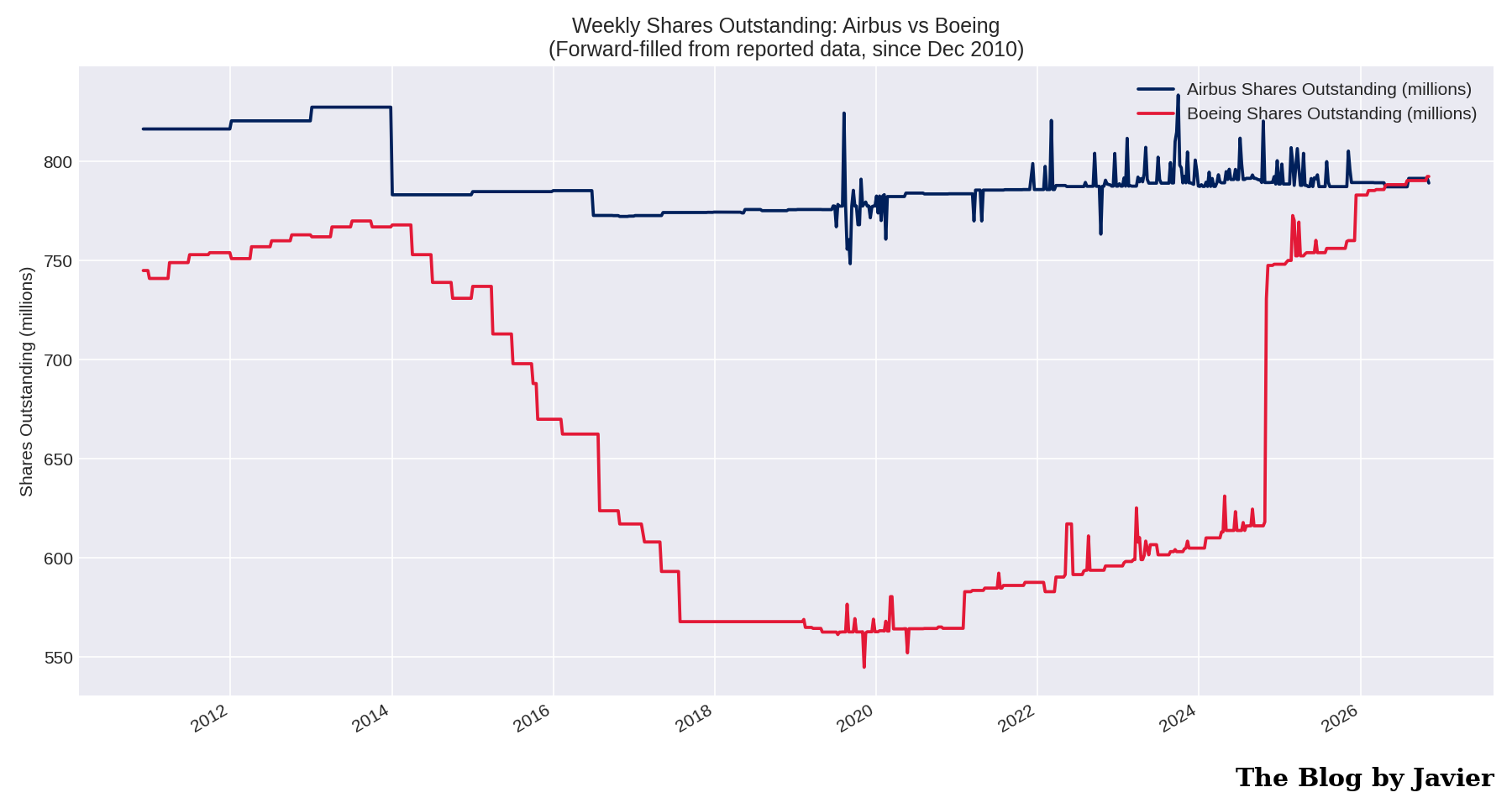
Weekly shares outstanding of Airbus and Boeing, forward-filled, since December 2010

Two opposite stories.

  • Airbus kept its share count roughly flat: ~816 million in late 2010, ~791 million today.
  • Boeing went from ~745 million down to ~545 million by November 2019 through share buybacks, and then back up to ~792 million after the capital raises of the last years. Boeing has today more shares outstanding than when the period started. More on this below.

Dollar-euro exchange rate

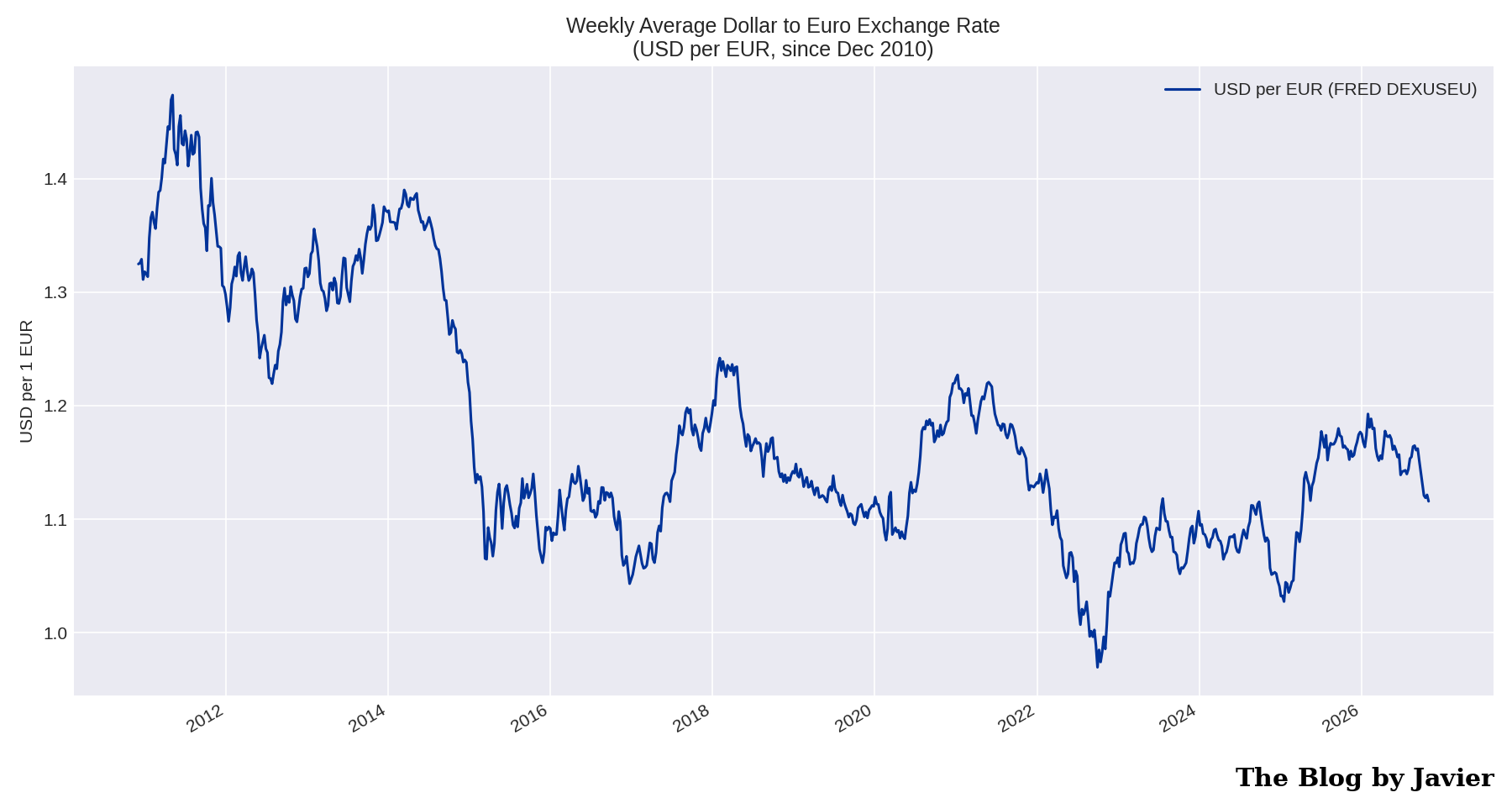
Weekly average USD per EUR exchange rate since December 2010

The euro went from ~1.32 dollars in December 2010 to ~1.12 at the end of October 2026, with a dip below parity in 2022. As Airbus reports in euros, the weaker euro weighs on the comparison in dollars: at a constant 2010 exchange rate, Airbus’ market capitalization in dollars would be about 15% higher than shown.

Market capitalization in US dollars

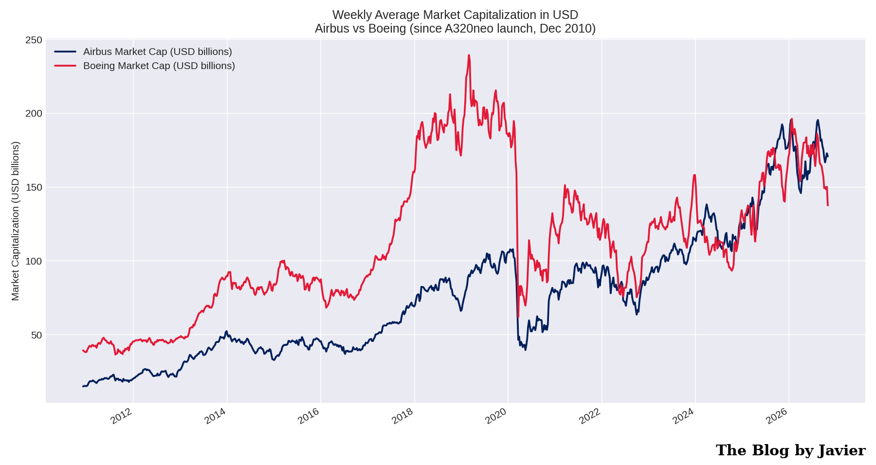
Weekly average market capitalization in USD billions of Airbus and Boeing since December 2010

This is the chart that puts it all together.

  • In early December 2010 Boeing’s market cap was ~$39bn versus ~$15bn for Airbus: Boeing was 2.6 times bigger.
  • Boeing peaked at ~$239bn in March 2019, weeks before the MAX grounding.
  • The first weekly close with Airbus above Boeing came in May 2022, and Airbus has been continuously ahead since late June 2026.
  • On 30 October 2026 Airbus stood at ~$171bn versus ~$138bn for Boeing, about 24% higher.
  • Averaged over the whole 16-year period Boeing was still the bigger company (~$113bn vs ~$75bn), which gives a sense of how large Boeing’s historical advantage was and how remarkable the reversal is.

Boeing share repurchases and dilution

As a final note of the 2024 post I left a link to a Leeham News and Analysis article with a contrarian view of Boeing’s stock buybacks. Its table of the 2013-2019 repurchase program is worth keeping here, now with the full historical context:

YearShares repurchased (millions)Value ($bn)
201325.42.8
201446.66.0
201546.76.8
201655.17.0
201746.19.2
201826.19.0
20196.92.7
Total252.943.5

The buybacks cut Boeing’s share count from ~745 million in 2010 to ~545 million by November 2019. Then came the 737 MAX grounding, the pandemic, the debt pile-up, and in October 2024, in the middle of a machinists’ strike, Boeing issued 129.4 million new shares at $143 (raising ~$18.2bn) plus $5bn of mandatory convertible preferred shares, as detailed in its SEC filings. The result: ~792 million shares outstanding today, more than before the buybacks began. The reduction that $43.5bn bought has been fully reversed, and then some.


Data sources

Leave a comment

Filed under Aerospace & Defence, Uncategorized

Marathon world record evolution (2026)

Last year I wrote an update of the all-time men’s marathon best times and the world record evolution (post here, following an older one from 2014, ahead of running that year’s Rotterdam marathon). This is a new update including 2026 best time as this has been an extraordinary year: the world record has been beaten and the two hours barrier has been broken in an official race for the first time in history. The 2026 version of the post includes all marathon times below 2h08′ up to and including today’s New York marathon.

As in the previous posts, I use the website “Track and Field all-time Performances” (maintained since years ago by Peter Larsson). As Larsson has not updated his marathon times list since mid August, this time I completed the dataset with World Athletics all-time toplists (which added 86 times from the races between late September and late October) and with today’s New York marathon results (from LetsRun, still provisional at the time of writing, as NYRR has not yet published the official ones).

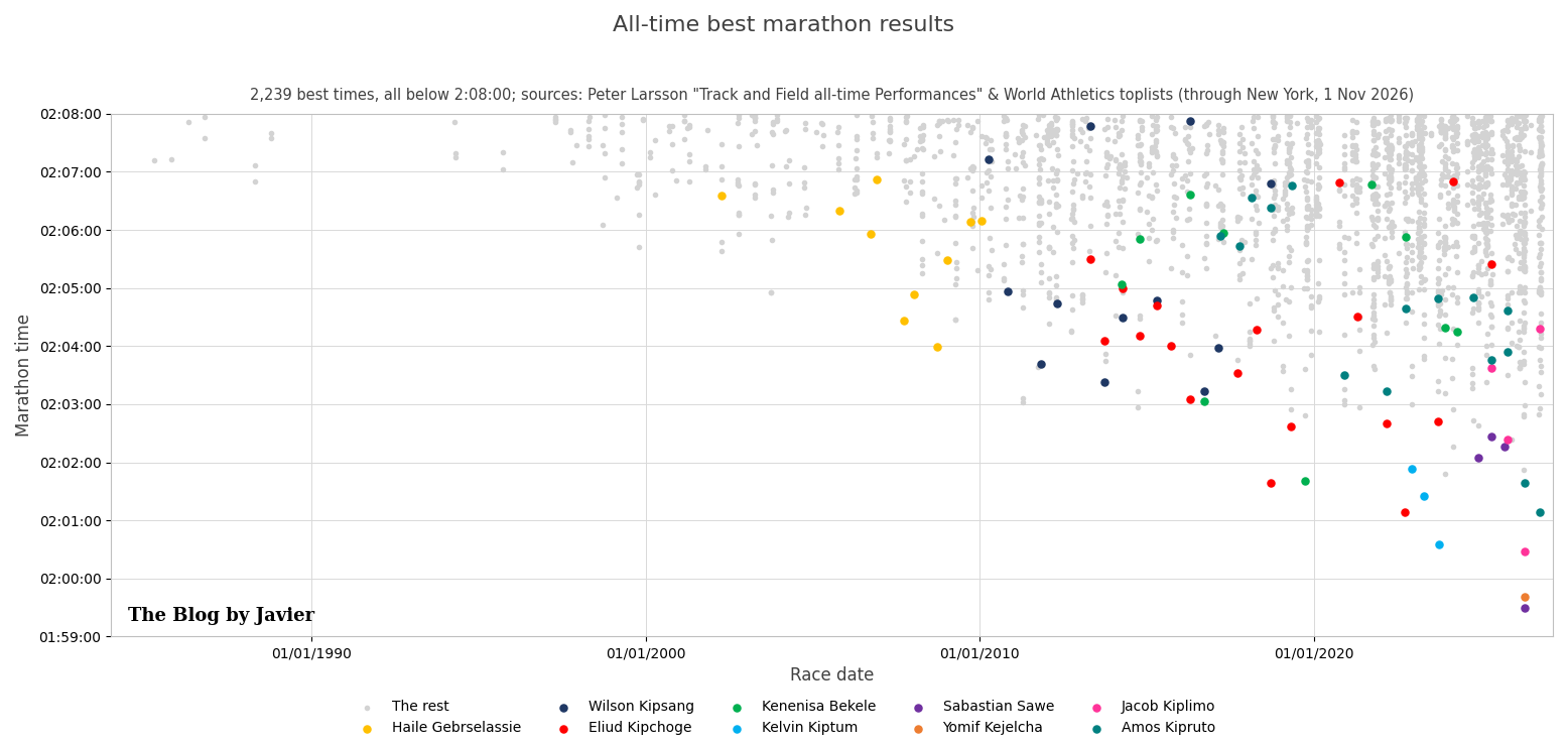
With the data of all-time best men’s marathon I plotted the chart below with the best 2,239 times, i.e., all those below 2h08′, and their dates, highlighting marathon times by Haile Gebrselassie, Wilson Kipsang, Eliud Kipchoge, Kenenisa Bekele, Kelvin Kiptum, Sabastian Sawe, Yomif Kejelcha, Jacob Kiplimo and Amos Kipruto.

All-time best marathon results, 2,239 times below 2h08

Some stats in relation to those 2,239 times under 2h08′ (they were 1,903 when I reviewed them in September 2025; 249 of them have been achieved in 2026 alone, more than in any previous year!):

  • Countries of which athletes achieved most such times: Kenya 959 times or 42.8%, Ethiopia 666 times or 29.7%, Japan 138 (6.2%), Morocco 51 (2.3%), Eritrea 51 (2.3%), USA 34 (1.5%), Uganda 27 (1.2%), Spain 27 (1.2%), Israel 26 (1.2%). Those are the top 9 countries, there are another 35 from which athletes have run below 2h08′ (for a total of 44 countries).
  • There are 872 athletes that have run below 2h08′. The individuals who have done so more often: Eliud Kipchoge 18 times (he still runs marathons, he even won the Melbourne marathon 3 weeks ago in 2h09 at 41 years old!), Sisay Lemma 17, Tamirat Tola 16, Amos Kipruto 15, Tsegay Kebede 15, Benson Kipruto 14, Abel Kirui 13, Evans Chebet 12, Wilson Kipsang 12, Geoffrey Kamworor 12, Bernard Kiprop 12, Birhanu Legese 11, … Kenenisa Bekele 10, Haile Gebrselassie 10…

Now, if we raise the bar to see the times at or below 2h05′, we find 301 times (they were 231 a year ago):

  • Countries of which athletes achieved most such times: Kenya 135 times or 44.9%, Ethiopia 121 times or 40.2% (both combined 85.1%!), Uganda 7 (2.3%), Tanzania 7 (2.3%), Belgium 5 (1.7%), Germany 5 (1.7%). Those are the top 6 countries, there are another 15 from which athletes have run at or below 2h05′ (for a total of 21 countries, 5 more than last year).
  • There are 154 athletes that have run at or below 2h05′ (30 more than last year). The individuals who have done so more often: Eliud Kipchoge 14 times, Amos Kipruto 10, Tamirat Tola 10, Wilson Kipsang 8, Sisay Lemma 7, Birhanu Legese 6, Gabriel Geay 5, Alexander Mutiso 5, Leul Gebrselassie 5, Sabastian Sawe 4,  Kenenisa Bekele 4, and several other athletes with 4, and with 3 times including Kelvin Kiptum, Dennis Kimetto, Geoffrey Mutai and Haile Gebrselassie.
  • Which are the fastest marathons? The cities where most of those 301 times at or below 2h05′ have been achieved are: Berlin 41, Valencia 39, London 33, Amsterdam 28, Dubai 27, Chicago 24, Rotterdam 22, Tokyo 21. Those are the top 8 cities (accounting for 78% of those 301 times), there are other 17 cities where such fast times have been achieved.

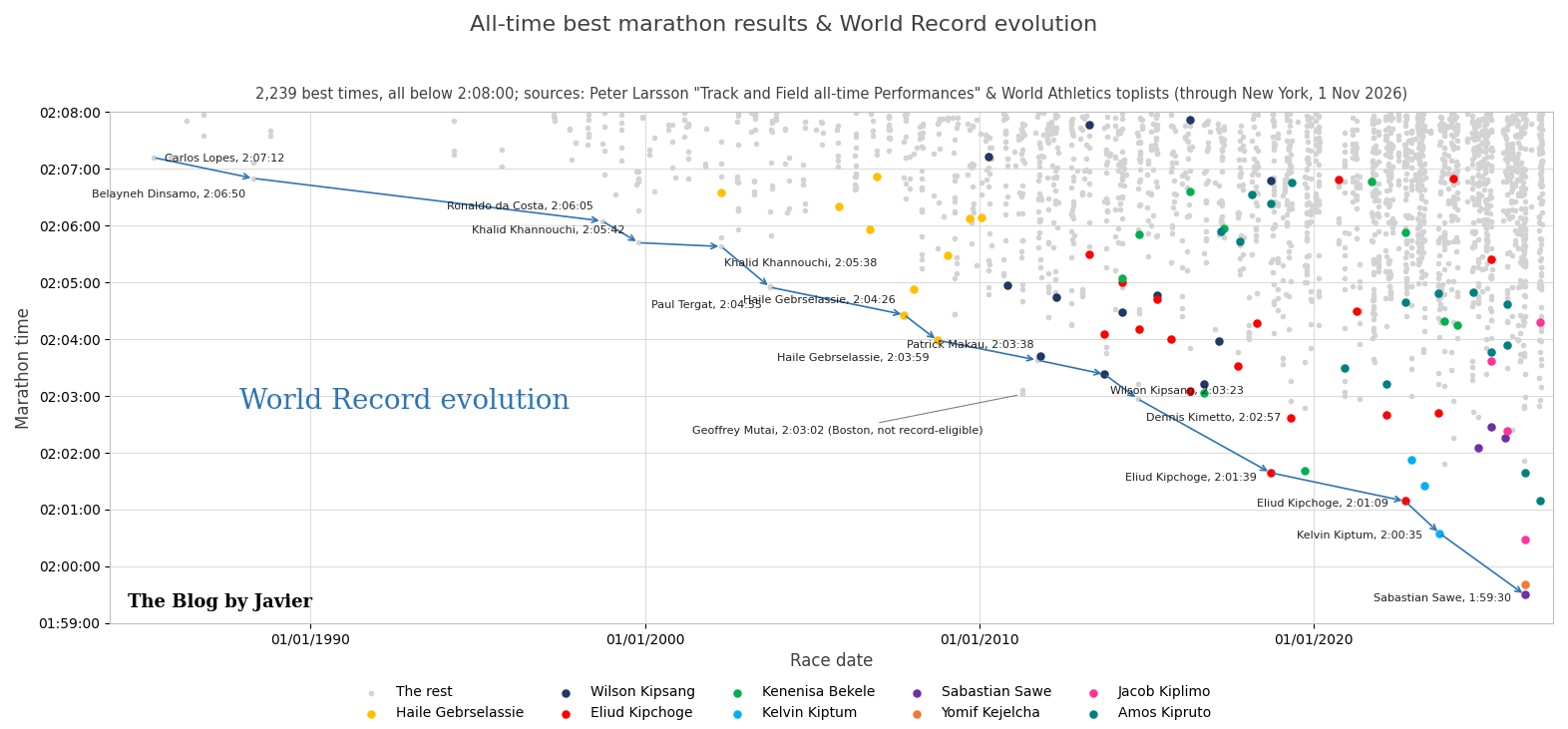
Now let’s look at the evolution of the World Record since 1985 in this other chart:

World record evolution since 1985, ending with Sawe 1:59:30 in 2026

Some comments to the chart:

  • In the last 41 years, the record has been beaten 14 times.
  • The current world record was set by Sabastian Sawe in London on 26 April 2026 with 1h59’30”, at the age of 31. It is the first official time below 2 hours and it was ratified by World Athletics in July (Eliud Kipchoge had run 1:59:41 in Vienna in 2019, but that exhibition, with rotating pacemakers, was not record-eligible).
  • That London race was historic beyond the record: Yomif Kejelcha (1h59’41”) and Jacob Kiplimo (2h00’28”) also finished under the previous world record, with Amos Kipruto 4th in 2h01’39”, Tamirat Tola 5th in 2h02’59” and Deresa Geleta 6th in 2h03’23”.
  • Sawe took 1’05” off Kiptum’s record, which had lasted two years and a half. The biggest improvement of the record was still made by Eliud Kipchoge, who took 1’18” off Dennis Kimetto’s previous record in 2018.
  • The record that lasted the most was Dinsamo’s 2:06:50 in 1988, which took just over 10 years to be beaten by Ronaldo da Costa in 1998.
  • 3 athletes have set the world record twice: Khalid Khannouchi, Haile Gebrselassie and Eliud Kipchoge.
  • Geoffrey Mutai ran in 2h03’02” in Boston 2011 and this year John Kipkosgei won Boston in 2h01’52”; as Boston is a downhill point-to-point course, those times do not count for the record.
  • In the same day in London, Tigst Assefa set a women-only world record of 2h15’41” (improving her own mark from 2025), with Hellen Obiri (2h15’53”) and Joyciline Jepkosgei (2h15’55”) completing the first race ever with 3 women below 2h16′ (see World Athletics report and London Marathon).

Other remarkable marathon facts from 2026:

  • Amos Kipruto won Chicago in 2h01’09”, equalling to the second the world record that Kipchoge had set in Berlin 2022.
  • Guye Adola won Berlin in 2h02’50”, and Tamirat Tola won Beijing in 2h03’10”.
  • Eliud Kipchoge, close to turning 42, ran won Melbourne two weeks ago.
  • Today in New York, Andreas Almgren (the reigning world half marathon champion) won in his marathon debut with 2h06’01”; 13 men ran below 2h08′.

What is the best age to run marathons?

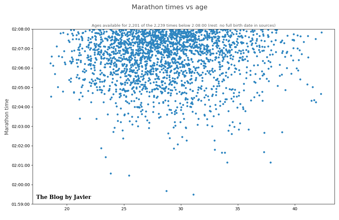
I plotted this other chart looking at the best 2,239 marathon times vs the age the runners had at the time of completing each of those races (for the 2,201 of them for which the sources include the full birth date).

Marathon times vs age

Most of the times below 2h08′ are achieved between 23 and 33 years old, and the very best ones are spread between 25 and 37, with the exceptions of the 3 marathons ran by Kelvin Kiptum, including his former world record at 23.9, Tadese Takele (2h03’24” at 21.1) and the 2h00’28” by Jacob Kiplimo at 25.4. Sawe’s world record, on the contrary, was set at 31.1. The youngest ever to run such a fast marathon was Tsegaye Mekonnen: 2h04’32” in Dubai 2014 at 18.6.

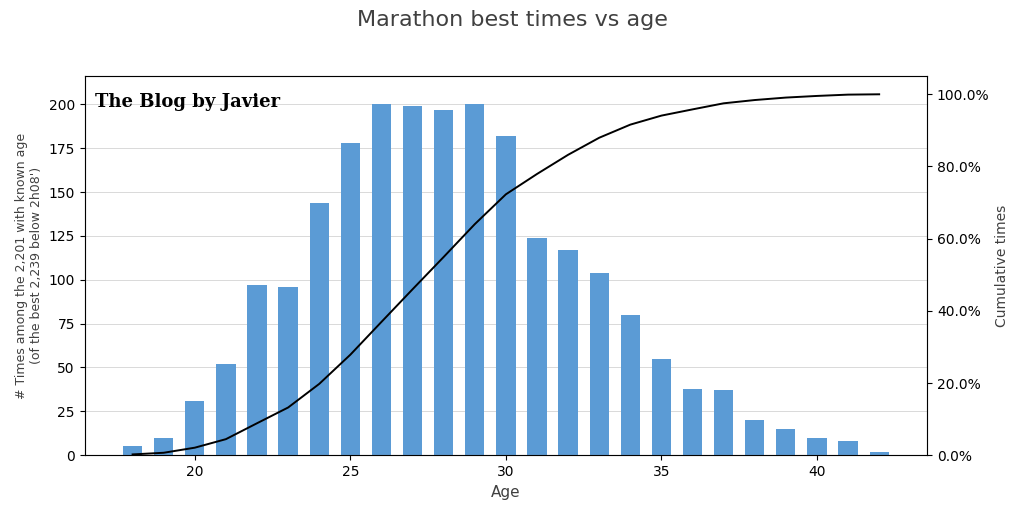
Another interesting chart to relate best times and age is the histogram below. In that one we can see that effectively most of the times below 2h08′ are achieved between 24 and 30 years old, and between 23 and 33 (both included) 79% of those times are achieved.

Histogram of marathon best times by age

Let’s see what Valencia brings in December with Yomif Kejelcha and John Korir on the roster.

Leave a comment

Filed under Sports, Uncategorized

El tren vive del contribuyente, el avión del pasajero: las cuentas del transporte en España

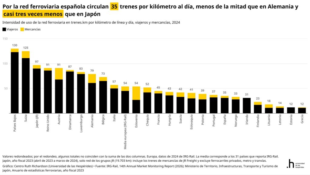
En estos días siguientes al terrible siniestro entre dos trenes de alta velocidad en Urda, varios opinadores señalaron a la liberalización del ferrocarril como una de las causas originarias debido al mayor uso de las vías, que haría más complicado su mantenimiento. Para rebatir esa línea argumental, en la red social X / Twitter, el profesor de la Universidad de las Hespérides Santiago Calvo publicó esta gráfica que muestra el todavía discreto uso de las vías de ferrocarril en España:

Pero esa discusión pública y otros comentarios, me sugirieron las siguientes preguntas: ¿Cómo de liberalizado está el sector del ferrocarril? ¿Cómo se compara con la aviación? ¿Cuánto dinero del contribuyente reciben unos y otros? ¿Qué incentivos hay?

Con la ayuda de los agentes de inteligencia artificial Grok e Instinct he preparado este post para ver algunos números que den respuesta a esas preguntas.

¿Cuánto dinero público reciben las grandes empresas públicas del transporte en España? Adif, Adif Alta Velocidad, Renfe, ENAIRE y Aena, de dónde vienen sus ingresos, cuáles ganan dinero y cuáles lo pierden. La respuesta, una vez vistos los datos de 2025, resulta incómoda para los defensores de la gestión pública: el ferrocarril se sostiene con miles de millones de euros de los contribuyentes cada año, mientras el sector aéreo se autofinancia por completo e incluso devuelve beneficios y dividendos al Estado. Lo público frente al mercado.

Quién es quién: propiedad y estructura

Las cinco empresas son públicas o de mayoría pública, pero con modelos muy distintos. Adif y Adif AV (Alta Velocidad) son entidades públicas empresariales del Ministerio de Transportes; Renfe y ENAIRE, sociedades mercantiles estatales; y Aena cotiza en Bolsa desde 2015, aunque el Estado conserva el 51 % a través de ENAIRE:

Del 49 % de Aena que está en manos privadas, los principales accionistas declarados hoy son el fondo activista TCI (The Children’s Investment Fund), con en torno al 6 % del capital total y BlackRock, que superó el 4 % en julio de 2025; el resto es free float repartido entre inversores institucionales y minoristas sin participaciones significativas declaradas. Los porcentajes son sobre el capital total (no sobre el 49 %) y corresponden a las últimas declaraciones de participaciones significativas a la CNMV recogidas en prensa en 2025.

EmpresaActividadPropiedadResultado 2025
AdifRed ferroviaria convencional100 % EstatalPérdidas: 83 M€
Adif Alta VelocidadRed de alta velocidad100 % EstatalPérdidas: 193 M€
RenfeTrenes de viajeros y mercancías100 % EstatalBeneficio: 60 M€
ENAIRENavegación aérea100 % EstatalBeneficio: 888 M€
AenaAeropuertos51 % Estado (ENAIRE); 49 % en Bolsa (TCI ~6 % y BlackRock >4 % del capital; resto, free float)Beneficio: 2.137 M€

¿E Iberia? La aerolínea de bandera dejó de ser pública hace 25 años: la privatización se decidió en 1997, en 1999 entraron socios industriales (British Airways entre ellos) y en abril de 2001 salió a Bolsa a 1,19 euros por acción. En 2011 se fusionó con British Airways para crear el grupo IAG (International Airlines Group) cuyo mayor accionista es hoy Qatar Airways, con un 25,1 %. Curiosamente, para preservar la nacionalidad española de Iberia (y sus derechos de tráfico), el 50,1 % de los derechos de voto de la aerolínea está en manos de Garanair, sociedad vinculada a El Corte Inglés. Iberia da beneficios y recibe regularmente premios por su puntualidad.

El ferrocarril: sostenido con miles de millones del presupuesto

El grueso de los ingresos del ferrocarril tienen como origen el bolsillo del contribuyente, por dos vías:

1. Los convenios con Adif y Adif AV. En julio de 2021 el Ministerio de Transportes firmó sendos convenios de sostenibilidad por los que ambas entidades percibirían 12.764 millones de euros entre 2021 y 2025: 8.747 millones para Adif (de ellos 2.539 de fondos europeos Next Generation) y 4.017 millones para Adif AV (2.154 de Next Generation). En la práctica, y según los datos de las cuentas anuales de 2025 depositadas en el Registro de la Intervención General de la Administración del Estado (cifras aún pendientes de contraste con las cuentas oficiales definitivas), solo en 2025 Adif recibió 2.468 millones de euros de dinero público (259 de subvenciones de explotación y el resto de capital para inversiones y aportaciones del accionista) frente a 633 millones que ingresó por su actividad; Adif AV recibió 1.257 millones frente a 789 millones de ingresos por cánones. Ambas pierden dinero: Adif cerró 2025 con 83 millones de pérdidas (el beneficio de 384 millones de 2024 vino de la venta de los terrenos de Madrid Nuevo Norte) y Adif AV con 193 millones, casi el doble que el año anterior, lastrada por una deuda de unos 18.300 millones que, tarde o temprano, pagarán entre todos los contribuyentes. Ninguna empresa privada podría operar así durante años sin que nadie responda por ello; en el sector público, en cambio, el agujero se cubre con el siguiente convenio.

2. Las compensaciones a Renfe por el servicio público. Cercanías, Media Distancia y Avant no se cubren con la venta de billetes: en 2025 esos servicios vendieron títulos por 532 millones y el déficit se paga con compensaciones de las administraciones. En total, Renfe contabilizó en 2025 1.851 millones de euros en subvenciones de explotación, que incluyen las compensaciones por las Obligaciones de Servicio Público del Estado y de la Generalitat de Cataluña y las bonificaciones de los abonos gratuitos. Gracias a ello, el grupo volvió a beneficios en 2025 por primera vez desde 2019: ganó 60,2 millones con unos ingresos totales de 4.480 millones, gracias sobre todo a los servicios comerciales de alta velocidad y larga distancia. El contrato-programa con el Estado sigue vigente hasta 2027, con compensaciones máximas de unos 916 millones al año.

El avión: un modelo que se autofinancia

La aviación funciona justo al revés: no vive del presupuesto, sino que aporta dinero al Estado. Y esto es porque hay una mayor liberalización, con multitud de empresas en competencia, lo que cambia por completo los incentivos: cuando una empresa (incluidas las públicas) se financia con lo que pagan sus usuarios, gestiona bien; cuando se financia con lo que paga el contribuyente, no tiene por qué hacerlo.

Aena se financia con las tasas aeroportuarias que pagan las aerolíneas y con sus ingresos comerciales (tiendas, restauración, aparcamientos). En 2025 ingresó 6.379 millones de euros y ganó 2.137 millones, un 10,5 % más que en 2024, con un EBITDA de 3.785 millones. Sus grandes inversiones (el plan DORA) salen del propio sistema aeroportuario, no de los Presupuestos Generales del Estado. Además, como el Estado conserva el 51 % a través de ENAIRE, la mayor parte de sus crecientes dividendos vuelven al Tesoro. No es casualidad que la gran empresa pública de transporte que funciona sea justo la que tiene un 49 % de capital privado en Bolsa que vigila sus cuentas cada trimestre. Sus subvenciones de explotación de 2025 fueron de 0,5 millones de euros; eso sí, conserva en balance 241,8 millones netos de subvenciones de capital concedidas históricamente, de las que imputa a resultados unos 25 millones al año.

ENAIRE, el gestor de navegación aérea, cobra tasas de ruta a las aerolíneas que cruzan el espacio aéreo español: 1.015 millones de euros en 2025, en torno al 85 % de sus ingresos. Es rentable: ganó 887,5 millones en 2025, de los que 737 vienen del dividendo de Aena, que acaba así en las cuentas públicas. Y apenas recibe dinero del Estado: 13 millones de subvenciones cobradas en 2025 (33,3 en 2024), principalmente fondos europeos MRR para modernización.

Las aerolíneas: el mercado que sí tiene competencia

Si el tren de alta velocidad tiene tres operadores (con sólo dos privados no pertenecientes al Estado español, Iryo (51% estado italiano, 25% Air Nostrum) y Ouigo (100% perteneciente a SNCF, ferrocarril estatal francés)), el cielo español es justo lo contrario: 180 aerolíneas operaron en el mercado español entre enero y diciembre de 2025, según la coyuntura del Ministerio de Transportes, y movieron 272 millones de pasajeros en vuelos comerciales (regulares y chárter; se cuentan las compañías con más de 1.000 pasajeros al año). Sólo 17 eran españolas, y transportaron 90,9 millones (el 33 % del total, un punto menos que en 2024); las 73 extranjeras comunitarias movieron 130 millones (el 48 %) y las 90 extracomunitarias, 51 millones (el 19 %).

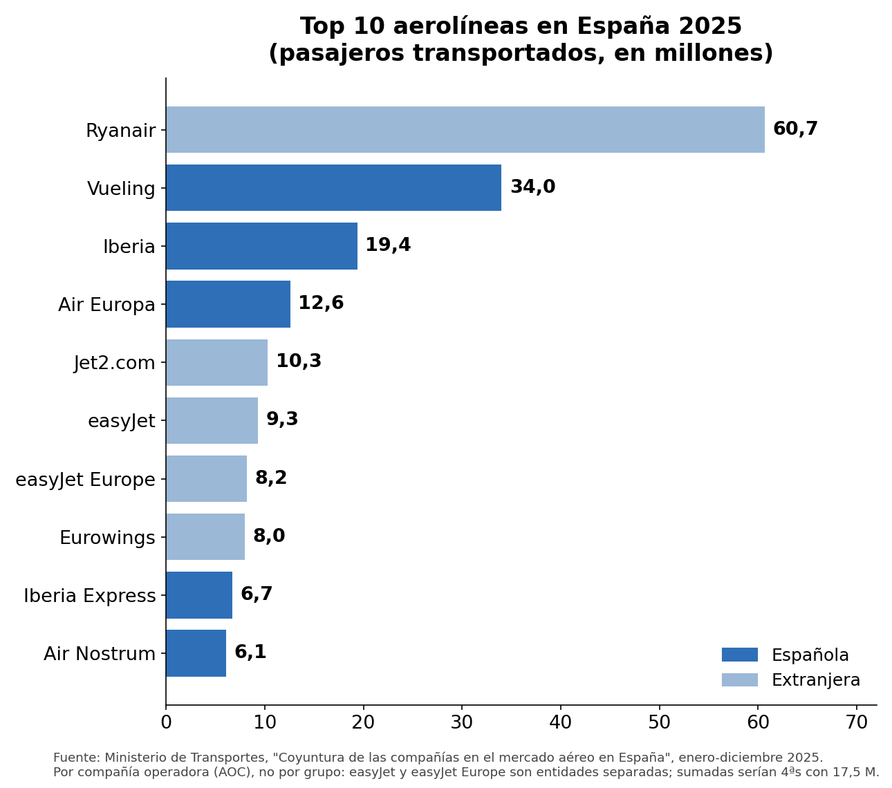
Top 10 aerolíneas en España 2025 en millones de pasajeros: Ryanair 60,7; Vueling 34,0; Iberia 19,4; Air Europa 12,6; Jet2.com 10,3; easyJet 9,3; easyJet Europe 8,2; Eurowings 8,0; Iberia Express 6,7; Air Nostrum 6,1. En azul oscuro las españolas, en azul claro las extranjeras.
Las diez aerolíneas con más pasajeros en el mercado español en 2025, por compañía operadora (no por grupo). Fuente: Ministerio de Transportes.

Las cinco primeras concentran la mitad del mercado: Ryanair lidera con 60,7 millones de pasajeros (+5,9 %), seguida de Vueling (34,0), Iberia (19,4), Air Europa (12,6) y Jet2.com (10,3). El ranking va por compañía operadora, no por grupo: easyJet y easyJet Europe aparecen por separado (sumadas serían cuartas, con 17,5 millones), igual que Iberia, Iberia Express y Air Nostrum forman parte del mismo grupo, IAG. La mitad de la tabla es española —Vueling, Iberia, Air Europa, Iberia Express y Air Nostrum— pero el líder destacado es irlandés. Es lo que tiene un mercado abierto y competitivo: precios bajos, récord de viajeros y empresas que se financian con lo que pagan sus clientes, no con el presupuesto.

Las ayudas del COVID: ¿se han devuelto?

Alguno podría argumentar “las aerolíneas también recibieron dinero durante la crisis del COVID” (cuando fueron impactadas por las prohibiciones y restricciones al transporte aéreo).

Durante la pandemia el Estado creó el fondo FASEE (Fondo de Apoyo a la Solvencia de Empresas Estratégicas, gestionado por la SEPI), que prestó 2.681 millones a empresas estratégicas, sobre todo aerolíneas privadas. Eran préstamos, no subvenciones, y se están devolviendo: Air Europa acaba de amortizar sus 475 millones (casi 500 con intereses) un año antes de lo previsto, y en total el fondo ya ha recuperado 1.425 millones, el 53 % de lo prestado.

Iberia y Vueling ni siquiera recibieron fondos del Estado, sino que suscribieron una serie de préstamos con distintos bancos privados (Santander, CaixaBank, Bankia, Bankinter, BBVA…) por valor de 1,010 millones de euros con aval del ICO (Instituto de Crédito Oficial). Esos préstamos se podían ir devolviendo hasta 2026, pero fueron amortizados en 2023, tres años antes de lo previsto.

Distinto es el caso de los fondos europeos Next Generation: son subvenciones a fondo perdido para inversiones, no hay nada que devolver, y sus principales receptores en el sector son precisamente Adif y Adif AV, con unos 4.700 millones previstos dentro de sus convenios.

La diferencia de fondo es elocuente: a las aerolíneas privadas se les prestó dinero que deben devolver, y lo están devolviendo; al ferrocarril público se le transfiere a fondo perdido, año tras año, sin fecha de caducidad ni obligación de rendir cuentas comparables. (La Fiscalía Europea investiga los fondos Next Gen)

Ferrocarril vs aviación, en tres métricas

Pedí a Instinct elaborar una gráfica con la proporción de ingresos “públicos” y “privados” de cada empresa, pero ese desglose no existe de forma comparable en sus cuentas: Adif no separa qué parte de sus cánones paga Renfe (pública) u Ouigo o iryo (privadas), Aena no distingue clientes públicos de privados, e “ingreso propio” no equivale a “ingreso privado” (las tasas de Aena y ENAIRE son cargas reguladas que fija la Administración, no precios de mercado puros). Lo que las cinco sí publican con criterios razonablemente parecidos (aunque no idénticos: unas son cuentas individuales y otras consolidadas, como indica el pie) es cuánto dinero público reciben al año, cuánto venden y cuánto ganan o pierden:

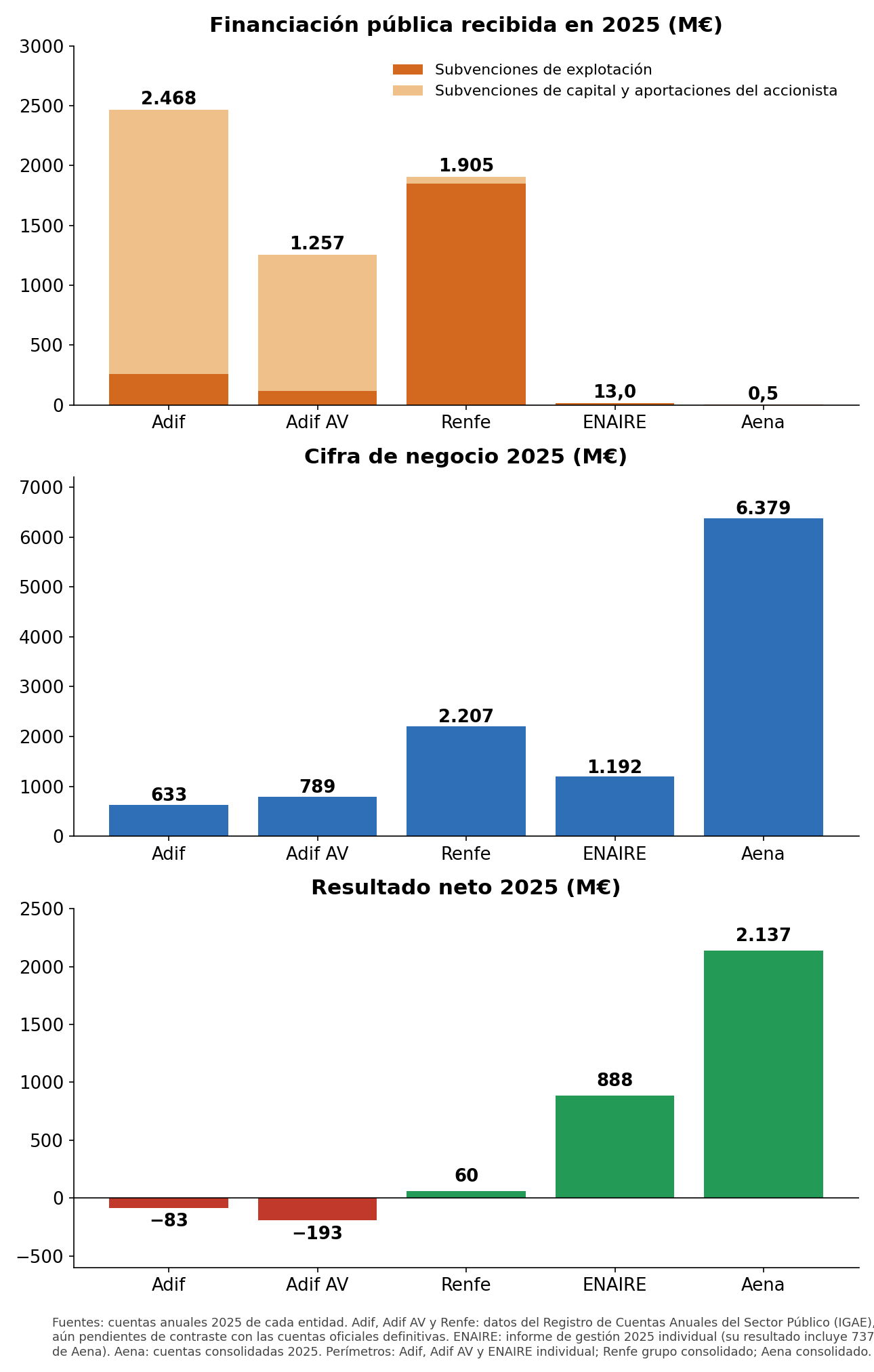
Tres paneles: financiación pública recibida en 2025 (Adif 2.468 M€, Renfe 1.905 M€, Adif AV 1.257 M€, ENAIRE 13 M€, Aena 0,5 M€), cifra de negocio 2025 (Aena 6.379 M€, Renfe 2.207 M€, ENAIRE 1.192 M€, Adif AV 789 M€, Adif 633 M€) y resultado neto 2025 (Aena 2.137 M€, ENAIRE 888 M€, Renfe 60 M€, Adif -83 M€, Adif AV -193 M€).
Financiación pública, ventas y resultado en 2025, en millones de euros. Las cifras ferroviarias del registro IGAE están pendientes de contraste oficial. Fuentes y perímetros en el pie de la imagen y en la sección de fuentes.

Tres lecturas:

  • Primera: la financiación pública se concentra en el ferrocarril; Adif, Adif AV y Renfe recibieron juntas unos 5.600 millones en 2025 (suma de tres transferencias estatales distintas, según los datos del registro aún pendientes de contraste oficial), mientras Aena y ENAIRE apenas registran subvenciones.
  • Segunda: la cifra de negocio aéreo supera con mucho a la del ferroviario.
  • Tercera: los resultados cierran el círculo; Aena y ENAIRE ganan dinero mientras Adif y Adif AV pierden 83 y 193 millones respectivamente.

En Adif y Adif AV la mayor parte del dinero público son subvenciones de capital que financian obras de la red, no gasto corriente; en AENA las obras en infraestructuras las paga el propio negocio. El tren es deficitario porque el legislador decidió que Cercanías y Media Distancia se presten como servicio público a precios que no cubren sus costes, igual que decidió que aeropuertos y navegación aérea se paguen con tasas a los usuarios. Las cifras exactas, con su documento y perímetro, están en las fuentes.

Ahora bien, mi lectura es la contraria a la conclusión de algunos opinadores: si hubiera más liberalización y no menos, las empresas (incluidas las públicas) del sector estarían mejor gestionadas y el sector florecería. Que el Estado decida financiar el ferrocarril es una mala idea pero legítima; lo que no lo es es que lo haga sin exigirle ni la disciplina ni la transparencia que el mercado impone al aéreo. Aena rinde cuentas cada trimestre ante accionistas privados y gana 2.137 millones; Adif AV acumula 18.300 millones de deuda sin que nadie responda por ella. Donde el AVE tiene competencia (Ouigo, iryo), el viajero ha ganado opciones y Renfe ha tenido que espabilar (y aún así compárese con la competencia del sector aéreo, incluido cómo compañías como Wizz y Ryanair acuden al rescate para conectar Madrid con Andalucía cuando se interrumpe el servicio ferroviario); donde no la hay, el contribuyente paga y calla. La pregunta que deberíamos hacernos no es cuánto más dinero público necesita el tren, sino por qué seguimos pagándolo sin exigirle las mismas reglas del juego que hacen viable al avión.


Fuentes:

Leave a comment

Filed under Aerospace & Defence, Economy, Uncategorized